2.2 Commodity Cluster - Another Message Passing Machine

We agree on the visionary raised by Culler et al. [32] and McColl [66] that the architectural trend of parallel computers is converging toward the following generic model - Most modern large-scale machines are constructed from general-purpose computers with a complete local memory hierarchy augmented by a communication unit, interfacing to a scalable network. This architectural insight includes a broad spectrum of parallel architectures, which ranges from Massively Parallel Processor (MPP) machine to the PC and workstation cluster. However, this conceptual architecture is too abstract for building up our communication model. As in our modeling framework, the architectural model lies on the lowest level, which needs to be a flexible and rich model that clearly delineates the performance capability of the target architectures.

2.2.1 Architectural Model

In our model, a cluster is defined as a collection of autonomous machines that are interconnected by two networks, one is driven by standard (STD) communication protocol such as TCP/IP, and the other is for high-performance communication that runs under the lightweight messaging protocol (LMP). Both networks can be comprised of same network technology, but normally the first one is running on a low-end LAN technology while the LMP network is on a high-performance LAN or SAN (System Area Network). Parallel applications running on the cluster make use of both networks. The LMP network is used primarily as the communication network for the parallel applications, while the STD network is used as the control/backup network, e.g. job submission and dispatching, as well as cluster management. For non-parallel applications such as sequential and distributed tasks, they only make use of the STD network if communications between machines are needed. Thus, our communication model is focusing on the performance characteristics of the LMP network under parallel applications.

All cluster nodes are assumed to have the same local characteristics, such as computation power, memory hierarchy, operating system supports, and communication hardware. In particular, we assume that each network adapter equips with one set of input and output channels, such that, it can simultaneously send and receive one data packet within one communication step. In general, parallel programs are programmed in SPMD (Single Program Multiple Data) mode, and follow the compute-interact mode of coarse-grained synchronization. As for the LMP network, it involves a global router/switch, interconnecting all nodes, and assuming a completely connected topology; hence, the network diameter between cluster nodes is not relevant under this architectural model.

For the global router, we assume that it supports an unreliable, packet-switched, pipelined network, and operates in full-duplex configuration under a fixed routing strategy. The logical unit of communication is packet, which is bounded to the range [1..MTUtypeset@protect @@footnote SF@gobble@opt MTU stands for the Maximum Transfer Unit of the communication system. ]. To transmit long messages, the system transfers them as sequences of packets. Packets generated from any given node travel along a predetermined fixed route through the network in order to reach their destination. To support completely connected configuration, the router has a deterministic delay in routing a packet from any input port to the destination output port in the absence of conflicts, but the overall performance is affected by the network load. Conflicts take place if more than one packet need to access the same output line, and are resolved by always forwarding the first arrived packet; the rest are buffered and routed later in a FIFO (First In First Out) manner. The amount of buffer memory inside the router is assumed to be finite, and therefore, the network can sustain certain level of congestion. Since we assume the network is unreliable, upon heavy congestion and the buffer space is exhausted, the router simply discards excess packets.

At first instance, this global router concept [70] seems to be an unrealistic assumption as this limits the scalability aspect of the cluster systems. However, current network technology allows us to scale the switching system to support hundreds to thousand of nodes interconnected by a single router switch with more or less uniform point-to-point latency. For example, both Extreme Networks [71] and Cisco Systems [98] claim that their high-end chassis switches, BlackDiamond 6816 from Extreme Networks and Catalyst 6500 series from Cisco Systems, can support up to 192 Gigabit Ethernet ports. In particular, the BlackDiamond switch can be configured to support at most 1440 Fast Ethernet ports with wire-speed Layer 2 and Layer 3 switching for consistent performance.

As we believe that an ideal abstract model must correspond to a programming model so that algorithms are designed or analyzed with the abstract model and coded in the programming model. With this architecture, the best-fit programming model would be the Message-Passing programming model, such that processes running in parallel are communicating with one another by sending and receiving messages. In a broader sense, all processes run in private address spaces and cooperate by means of explicit message exchange. Therefore, to delineate the association between the abstract model and programming model, we draw our attention on how data are moving over this architecture.

2.2.2 Data Transfers

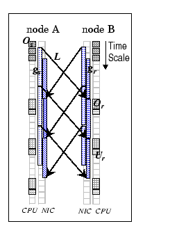
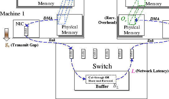
The data transfers have a significant impact on the communication performance, so optimizing this critical path is essential to obtain high-performance, and this becomes the main objective of all lightweight messaging systems. Despite of the vast difference in implementation choices and target network technologies, we observe that data transmissions are commonly going through three phases, from sender address space to receiver address space. A typical scenario would look as follows: the data on the sender side first traverse through the send phase, which is usually under the control of the host processor. Then the messages are delivered by the network hardware (network interface cards (NICs) and switches) to the other end during the transfer phase of the transmission. Eventually, at the other end, the receive phase terminates this transmission by delivering the data to the corresponding receive process.

2.2.2.0.1 Send Phase

This phase includes all events happened before the network adapter takes over the control in handling the data transfer. We consider this phase starts from the time when the user process is ready to send its message, to the time when the data message is transformed to a hardware dependent format that is ready to be transmitted by the network adapter. With traditional communication protocol, this includes system call handling, cross-domain data copying, checksum computing, protocol stacks traversing, and other processing overheads. However, for all lightweight messaging systems, all those unnecessary overheads have been removed so as to shorten the software gap between the user process and network hardware. Regardless of the optimization techniques used in this phase, all LMP systems must take care on how to ``move'' the data message from the sender's memory space to the network adapter's address space.

One major difference between these lightweight messaging systems is the obligation of the host processor with respect to the multiplexing task. To support multiprogramming, the LMP systems are required to efficiently multiplex multiple message streams, and deliver these intermixed data packets to the corresponding destinations. For network adapters with a programmable communication co-processor, some LMP systems off-load the multiplexing task to the co-processor. This allows the host processor to do other computation, and thus, effectively reduces the software overhead. On the other hand, without the help from a communication processor, the multiplexing task becomes the sole responsibility of the kernel due to the protection and integrity reasons, and therefore, the observed software overhead would be higher.

For example, BIP [83] is a user-space communication library built on top of the Myrinet network [15]. To deliver near raw speed performance (i.e. the achieved one-way latency is 4.3 $\mu s$ for an empty message), it simply exposes the network interface to a single user-space process and relies solely on the Myrinet hardware for the reliability. On the other end, PM [101] is another user-space communication library running on Myrinet; it supports multiprogramming as well as adopting flow-control mechanism to avoid receive-buffer overrun. Same as BIP, it relies on the Myrinet hardware to guarantee the data delivery between NICs. Its one-way latency is 7.2 $\mu s$ for an 8-byte message. Therefore, we reckon that the overall cost of this send phase could become a performance index, which reflects the functionality of the lightweight messaging protocol as well as the processing capability of the network hardware.

2.2.2.0.2 Transfer Phase

The transfer phase is wholly a network-dependent part. This phase involves all the events happened in transporting the data through the network to the remote peer. In general, this includes two DMA transfers, one in the host node and the other in the remote node, together with the physical transmission of the data through the wires and switches. Factors attribute to the movement cost of this phase are:

• The I/O bus bandwidth, e.g. PCI, VME, MicroChannel, SBus, etc. For example, Tezuka et al. [101] have reported of the significant difference in the measured network bandwidth between SBus and PCI bus on the Myrinet networks that were driven by the PM protocol.
• The network transmission speed, e.g. 100 Mb/s with Fast Ethernet, 1 Gb/s with Gigabit Ethernet, 2 Gb/s with Myrinet-2000, 10 Gb/s with 10 Gigabit Ethernet, etc. The higher the transmission speed, the shorter the network delay.
• The network interface protocol or firmware, e.g. Myrinet-interface control program, QsNet driver, etc. With the use of programmable network interfaces, more functions can be included, e.g. address translation and reliable support, which significantly reduces the software overhead. On the other hand, this increases the network delay when more complex network interface protocol is used, e.g. AM II [23].
• The network topology, e.g. multistage interconnection network, crossbar network, irregular network, etc. This affects the distance or diameter between the cluster nodes, which in turn affects the transmission delay on the network.
• Underlying switching technique, e.g. store-and-forward switching, virtual cut-through switching, wormhole switching, etc.

It is a non-trivial task to capture all these factors as one has to know all the details of the underlying hardware, which overwhelms the performance understanding process.

Despite of having many factors contribute to the transfer cost, the prevailing factor is the network technology to which these LMP systems are targeting. This is because once we have decided on the network technology, we are confined to the technological constraints of the underlying network. For example, performance of the network is more heavily influenced by the switching technique than by the topology or the routing algorithm [35]. However, most of the Fast Ethernet or Gigabit Ethernet switches are using store-and-forward packet switching. Therefore, those LMP system running on these networks are known to have higher network delay, albeit supporting a larger non-blocking network. In contrast, the Myrinet switches are using wormhole switching, we are therefore expecting a very low hardware latency, e.g. 0.1$\mu s$ per switch latency [69], which significantly improves the point-to-point communication performance.

Besides of the hardware delay, the adopted switching technique also affects the way in which the switch handles network conflict. For examples, store-and-forward switch uses buffer queue to store the whole packet, while wormhole switch applies link-by-link flow control to stall the transmission instead of buffering the packet. Although these two techniques both increase the network delay, they give completely different impression to the end-user. For the store-and-forward buffering, the end-user would experience an increase in the per packet network delay, while for the wormhole switching, the end-user would experience an increase in per message injection rate. Nevertheless, these minor differences may affect the design choice in devising efficient communication algorithms.

2.2.2.0.3 Receive Phase

This phase includes all events happen at the destination node when message is handed over by the network adapter, until it is being dispatched to the corresponding receiver's process space. It looks as if the receive phase is just the opposite of the send phase, but it is not. In the data transfer event, message reception is an asynchronous event as receiving process does not know when will a message arrive. To dispatch the data to the right place, i.e. the reverse of multiplexing, the system needs to know where the data should go. This has to be managed by a privilege process that gets hold of those protected informations, and this becomes the major difference between different LMP implementations. For those LMP systems that do not make use of any communication co-processors, this becomes the sole responsibility of the operating system. To notify the kernel on the message reception, the network adapter needs to raise a hardware interrupt. However, interrupts are high priority events, they have great performance impact on modern CPU architecture, such as flushing pipelines and reducing cache locality.

Even though with the availability of communication co-processor, different LMP systems take different strategies on the message reception. Some LMP do not take advantage on the co-processor, and use the in-kernel approach, e.g. AM-II [23] and FM [75]. Others program the co-processor to move the incoming message directly to a pre-pinned and pre-translated user-space address, e.g. PM [102] and LFC [12], or using a more aggressive approach that integrates a translation look-aside buffer into the network interface to pin and translate user-space addresses dynamically, e.g. UNet/MM [115]. Moreover, no matter which protocols they are using, the performance of this phase is greatly affected by the processing speed of the protocol processor, the lightweight messaging protocol, and the I/O bus bandwidth. It is found that this phase is most likely to be the bottleneck of the whole transmission path, especially if the processing speed is not fast enough to drain-off all incoming messages.

$\;$

Table 2.2: Breakdown analysis of several lightweight messaging systems with respect to the three-phase data transfer. During the data transfer, we assume that the outgoing message is resided on any virtual address space of the sender process, and is going to be delivered to any virtual address space of the receiver process.

	AM II [23]		FM2.x [58]	BIP [83]		PM1.2 [101]	UNet/ATM [108]
pre-communication setup	endpoints creation		context creation		context creation	endpoints creation
possible per-communication overhead	endpoint faults			pin send & receive buffer		gang scheduling overhead	copy-to-DMA
			synchronize on long message		pin-down cache overhead
send phase	library call		library call	library call		library call	library call
	Short: PIO	Long: copy-to-DMA	acquire device lock	Short: PIO			PIO metadata
	receive polling		PIO with write combine
transfer phase	endpoint management overhead		Myrinet transfer		DMA to NIC	DMA to NIC	DMA to NIC
		DMA to NIC	DMA from NIC	Myrinet transfer		Myrinet transfer	ATM transfer
	Myrinet transfer				DMA from NIC	DMA from NIC	DMA from NIC
	endpoint management overhead
		DMA from NIC
receive phase	polling or interrupt		polling	polling		polling	polling
	PIO	copy-from-DMA	copy-from-DMA	PIO		copy-from-DMA	copy-from-DMA

$\qquad$

	GigaE-PM2 [95]	GAMMA [22]	DP	UNET/FE [114]
pre-communication setup	context creation	active port setup	DP endpoint creation	endpoint creation
possible per-communication overhead	acquire send buffer	pin send & receive buffer		copy-to-DMA
send phase	copy-to-DMA	lightweight system call	lightweight system call	lightweight system call
	system call		copy-to-DMA
transfer phase	DMA to NIC	DMA to NIC	DMA to NIC	DMA to NIC
	GE or FE transfer	GE or FE transfer	GE or FE transfer	FE transfer
	DMA from NIC	DMA from NIC	DMA from NIC	DMA from NIC
receive phase	interrupt or polling	interrupt	interrupt	interrupt
	copy-from-DMA	copy-from-DMA	copy-from-DMA	copy-from-DMA
	copy-to-user		copy-to-user	copy-to-user

To summarize, we present a breakdown analysis of several user-level or kernel-level lightweight messaging systems in Table 2.2, and categorize their activities with respect to the three-phase data transfer. We observe that different LMP systems have different massing-passing semantics and implementations, and this is being reflected by the differences in involvement within the three phases. However, their events or activities are generally captured by this three-phase data transmission scenario.

2.2.3 The Communication Model

A practical way to understand the performance characteristics of a parallel program on a parallel architecture, is to look from a processor's viewpoint at the different components of time spent executing the program [32]. With each component of time spent reflects the software-plus-hardware performance of a specific architectural feature, a collection of these components becomes a set of performance indices that related directly to the performance understanding issues. In the previous section, we have laid out the architectural model of the cluster platform as well as the typical scenarios involved in moving data over this architecture. Since data communication lies on the critical path of a message-passing machine, the straight-forward way in performance understanding is to identify abstract components that characterize this critical path - the data transfer.

To characterize the transfer, a communication model is associated with our architectural model, which delineates the costs induced by moving the data around, both locally and remotely. We consider data communication via the network as an extension to the memory hierarchy concept, such that it is a data movement from the remote memory region to the local memory region, or vice versa. There may have two types of data movements in a communication event: a) remote data transfers and b) local data transfers. It is important to include the local data transfer abstractions to our performance model. This is because, in the associated message-passing model, we are not restricting on the ``whereabouts'' factor of the data messages. Since data messages can be resided in anywhere of a process address space, and some communication systems require the placement of these data messages be in some pre-defined memory region, e.g. UNet and GigaE-PM2, thus, local data movements are included so as to accomplish this programming abstractions.

Remote Data Transfer

We encapsulate all the overheads of the three-phase data transfer by a set of model parameters, and below are the detail description of individual parameters. The associated microbenchmarks for deriving the cost functions of this parameter set are provided in Appendix A. In addition, Figure 2.1 summarizes this abstract model as a schematic drawing that delineates the relations of different performance parameters to the architectural model.

Figure 2.1: Model parameters affiliated with the remote data transfer

2.2.3.0.0.1 Machine size p

This refers to the number of processes participating in this communication event.

2.2.3.0.0.2 Send overhead $O_{s}(m)$

This parameter stands for the software overhead associated with the send process for sending an m-byte data packet. From the high level perspective, we view it as the time used by the user process to interact with the logical network interface, prepare the message, forward the message to the network adapter, and signal the network hardware. Therefore, it encapsulates all the events happened in send phase. This parameter captures several performance features of the communication system, such as the speed of the host processor, the efficiency of the memory subsystem, and the lightweight messaging protocol in use. We model this parameter by a simple linear function,

$$O_{s}(m)=\kappa _{s}+\tau _{s}m$$ (2.1)

where $\kappa _{s}$ is the startup cost of this event which depends on the node processing power, m is the message length bounded by the range [1..MTU], and $\tau _{s}$ is the data transfer rate that depends on the efficiency of the memory subsystem. Subject to the particular LMP protocol, for example, under zero memory copy, this linear function can be reduced to a simple constant, i.e. $O_{s}(m)=\kappa _{s}$. As this is a synchronous event, we quantify this parameter by directly measuring the time engaged by the processor in handling those activities.

2.2.3.0.0.3 Inter-packet transmit gap $g_{s}(m)$

Owing to the difference in data movement speeds between the send and transfer phases, the network hardware is moving data packets with a confined capacity, which is captured by this parameter. For example, the performance of the I/O bus and the network technology are the major factors of this parameter. This inter-packet gap has two slightly different meanings with respect to different perspectives, but in general, it delineates the maximum network throughput available to the user process. From the user process perspective, it views the gap as the minimum service time of the network in transmitting consecutive data packets. Thus, any attempt to send data faster than this gap yields no performance gain, and the difference between $g_{s}$ and $O_{s}$ indicates the amount of CPU cycles available for the processor to do other useful computation or perform the receive operation during bidirectional communication. From the network perspective, it represents the maximum injection rate of the packets to the network. This parameter is delineated as

$$g_{s}(m)=g_{1}+\tau _{1}m$$ (2.2)

where $g_{1}$ stands for the startup cost necessary to initiate the transfer and $\tau _{1}$ reflects the available communication bandwidth provided by the I/O bus and the network.

2.2.3.0.0.4 Network latency $L(m,p)$

This parameter represents the time used by the network to move an m-byte data packet from the physical memory of the source node to the physical memory of the destination node. It is a network-dependent parameter, which encapsulates the performance of the host I/O bus, the network topology, the network technology and the network interface protocol (or firmware) in use. Since we model the network as a complete graph, the topology and the distance factors can be eliminated. In general, the value of L is subjected to the traffic loading at any particular instant in a real network. For example, when routing the packets through the network, conflicts take place if more than one packet accesses the same output line, and temporary buffering is needed. This delay affects the overall network performance perceived by the users. The amount of buffer memory inside the switch is assumed to be finite, thus, the network can sustain certain level of congestion. We model this phase by a bilinear function under the congestion-free condition,

$$L(m,p)=l(p)+m\tau _{L}(m,p)$$ (2.3)

where $l(p)$ is a function representing the cumulative startup cost of this network transfer and $\tau _{L}(m,p)$ is the available network throughput. Both l and $\tau _{L}$ are a function of p. Routing a packet involves utilization of some central resources (e.g. buffer control unit and forwarding control unit), therefore, contention for resources may occur if more than one routing request happen concurrently. The extent of this contention is subjected to the switch internal architecture, and different routers may behave differently. Some networks may only have limited aggregate bandwidth, they cannot service too many communicating pairs at a time and contention arises. So the allocated network throughput to the transfer phase depends on the aggregate bandwidth of the network, the number of communicating pairs and the volume of the communication, thus, $\tau _{L}$ is a function of both p and m.

2.2.3.0.0.5 Inter-packet receive gap $g_{r}(m)$

This parameter stands for the minimum time interval between two consecutive receptions experienced by the receiving host, which is limited by the performance of the I/O bus and the network technology in use. Similar to the $g_{s}$ parameter, it is used to delineate the maximum packet arrival rate delivered by the network or the maximum service rate of the network hardware. This parameter has two uses. First, the inter-packet receive gap reflects the CPU cycles available to handle arrived packets, so this information should be taken into consideration during LMP design. For example, should we implement an address translation mechanism to support true ``zero-copy'' on the receive path, or simply using a one-copy semantic? We can make use of the receive gap parameter to justify on various design trade-offs. Second, as we cannot receive more than one packet within the receive gap, this information is particularly useful in designing communication schedules. For example, we can use this information to schedule a collective operation, which involves both send and receive events.

Same as the $g_{s}$ parameter, this receive gap is captured by a linear function,

$$g_{r}(m)=g_{2}+\tau _{2}m$$ (2.4)

For simplicity, on a homogeneous cluster, we can generally assume $\tau _{1}=\tau _{2}$, as both are related to the transfer capability of the network and the I/O bus.

2.2.3.0.0.6 Network buffer capacity $B_{L}$

Resource contention is the major cause of congestion, which in turn, affects the delay experienced by the applications. In reality, congestion is a fact that we need to face with. The $B_{L}$ parameter corresponds to the available buffer capacity in the global router, which is a measure of the network tolerance of the router in handling contention. For a router/switch, we only have one $B_{L}$ value, either it is associated to the whole switch if it is a shared-buffered switch, or is associated to a switch port if it is an input-buffered or output-buffered switch. By capturing the finite capacity of the network buffers, algorithm designers can calculate the network endurance, and avoid congestion loss with appropriate communication schedules.

2.2.3.0.0.7 Asynchronous receive overhead $O_{r}(m)$

This parameter captures the software overhead in handling incoming messages. As there is no central coordination between communicating parties, and the messages can be arrived at anytime on packet-switched network; thus, message reception is considered as an asynchronous event which does not involve the receiving process. This parameter captures the costs of all kernel events including interrupt, memory copy and context switch, and its efficiency is affected by the processing speed of the processor and the lightweight messaging protocol in use. In our model, we express it as a linear equation,

$$O_{r}(m)=\kappa _{r}+\tau _{r}m$$ (2.5)

In which $\kappa _{r}$ represents the minimal cost of this asynchronous event, such as interrupt cost, buffer management, and protocol overhead; while $\tau _{r}$ mainly reflects the speed of memory movement between different memory regions if needed.

2.2.3.0.0.8 User receive overhead $U_{r}(m)$

Due to the asynchronous nature of the communication, the receiving process needs to find some means to check for data arrival, e.g. polling, block & wake-up by signal, or hybrid approaches; and consumes the data, e.g. copy to other memory segment. This parameter reflects the software overhead spent by the receiving process after arrival of packets. In most of the performance evaluation reports, due to the artificial nature of the benchmark programs, this parameter is of insignificantly low cost. However, in reality, this overhead reflects the performance loss due to improper coordination of communication events. For example, in a multi-user environment, polling is a user-level event that is affected by the regular CPU scheduling policy. If the receiving process cannot be scheduled frequently to poll for its data, the overall performance may degrade significantly.

Local Data Transfer

$\qquad$

2.2.3.0.0.9 Memory copy overheads $M_{ctc}$, $M_{ctm}$, & $M_{mtm}$

Memory copy issue has been extensively studied in the past, and is being classified as a high overhead event. To avoid this overhead, most of the low-latency communication systems have removed it from their protocol stacks. However, in reality, memory copy operations cannot be avoided completely. For example, some high-level communication schemes such as Gather and All-to-all, require to have the resulting messages be returned in contiguous memory buffer. Thus, extra memory copy operations are needed. To quantify these costs, we provide three memory copy parameters - $M_{ctc}$, $M_{ctm}$, and $M_{mtm}$ to represent the costs induced by data movement between different memory hierarchies, such as the cache-to-cache, cache-to-memory, and memory-to-memory data movement.

2.2.4 Simple Examples

2.2.4.0.1 Point-to-point communication

For a homogeneous cluster, we generally assume that $g_{s}\approx g_{r}$ and simplify the expression by $g=\max (g_{s},g_{r})$. To take advantage of the full-duplex communication, we assume that the cluster communication system satisfies this condition, $(O_{s}+O_{r}+U_{r})<g<L$. This assumption is generally true under the current microprocessor technologies and the adoption of low-latency communication. As a result, under no conflict, the one-way point-to-point communication cost ($T_{p2p}$) in transferring an M-byte ``long'' message between two remote user processes is:

$$T_{p2p}(M)=O_{s}+(k-1)g+L+O_{r}+U_{r}$$ (2.6)

where $k=\frac{M}{b}$, which corresponds to the fragmentation of an M-byte message to k data packets of size b bytes. For optimal performance, b usually stands for the maximum transfer unit (MTU) of the underlying network technology.

Figure 2.2: Point-to-point communications with $(O_{s}+O_{r}+U_{r})<g$

[uni-directional flow] [bi-directional flow]

Similarly, the bi-directional exchange communication cost ($T_{xchg}$) between two nodes can be expressed as:

$$T_{xchg}(M)=O_{s}+(k-1)g+L+O_{r}+U_{r}$$ (2.7)

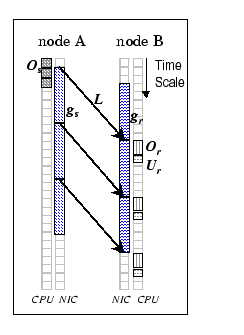
It is interested to see that both one-way and two-way exchanges have the same cost. Figure 2.2 presents the graphical breakdown of these point-to-point communications and shows that when full-duplex condition is met, both send and receive phases can be happened concurrently without interfering each other. Although $O_{r}$ is a high-priority event which always preempts other activities, as we have $(O_{s}+O_{r}+U_{r})<g$, the processor is capable to perform both send and receive activities within one $g$ interval. Thus, we see that the bottleneck of the communication falls on the network component. In theory, their costs would remain the same as long as the bi-directional network throughput is within the I/O bus throughput constraint. The next example will focus on how the assumption of the full-duplex condition affects other high-level communication issue.

2.2.4.0.2 Broadcast operation

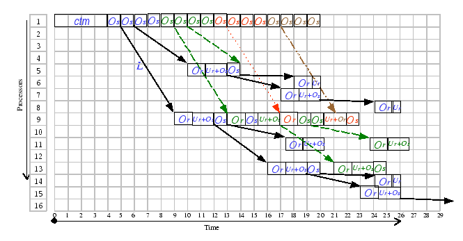
This one-to-many communication pattern appears in many parallel and distributed applications, thus, it is included in most of the high-level massage-passing libraries, e.g. MPI. Most of these libraries implement the broadcast operation on top of the point-to-point primitive with the tree-based algorithm. To broadcast a long message of size M bytes (larger than the MTU), we simply repeat the broadcast algorithm $\frac{M}{MTU}=k$ times. Based on our communication model, we have graphically constructed this broadcast communication tree and present it in

Figure 2.3: Tree-based broadcast operation expressed in our model terminology with $p=16$, $L=4$, $g=2$, $O_{s}=1$, $O_{r}=1.5$, $U_{r}=0.5$; however, the full-duplex constraint cannot be satisfied.

Figure 2.3. The corresponding cost formula expressed in our model terminology is:

$$\textstyle B_{k}(p) = ctm(M)+O_{s}+g(k-1)log_{2}p+(L+O_{r}+U_{r}+O_{s})log_{2}p-O_{s}$$

$$= ctm(M)+log_{2}p\left( (k-1)g+L+O_{r}+U_{r}+O_{s}\right)$$ (2.8)

The above formula models the communication cost of sending an M-byte message that resides in an arbitrary virtual address on node 1 to p-1 nodes. Although, with this parameter set, the full-duplex condition is not reachedtypeset@protect @@footnote SF@gobble@opt $U_{r}$ includes an $mtm$ copy so as to reconstruct an M-byte message before forwarding to the user process , we find that there is no interference between the send and receive events. In addition, we notice that the broadcast root is the bottleneck of this communication schedule. Nevertheless, since no interference exists, this derived cost formula should cover other cluster configurations that satisfy the full-duplex condition.

Figure 2.4: The same broadcast schedule on another cluster configuration with g reduced from 2 to 1

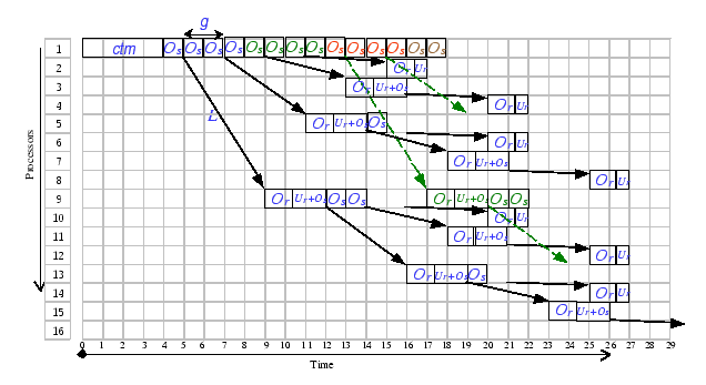
Figure 2.4 delineates the same broadcast tree that works on a different cluster, which exhibits different characteristics. From this broadcast tree, we identify that the bottleneck region of this broadcast pattern is at the $\frac{p}{2}^{th}$ processor, but not at the broadcast root. Of the previous broadcast communication schedule (Figure 2.3), we find no interference exists in successive broadcast, such that the reception of the $i^{th}$ packet does not overlap with the transmission of the $(i-1)^{th}$ packet to its subtree. But under the new cluster setting, as shown in Figure 2.4, at processor 9 - the $\frac{p}{2}^{th}$ processor of this broadcast event, the transmission of the $i^{th}$ packet is always overlapped with the reception of the $j^{th}$ packet for any $j>i$. With this observation, the new cost formula of this broadcast pattern under this new cluster setting becomes:

$$\textstyle B_{k}(p) = ctm(M)+O_{s}+L+(k-1)\cdot \left( O_{r}+U_{r}+\left( log_{2}p-1\right) O_{s}\right)$$

$$\: +O_{r}+U_{r}+O_{s}+(log_{2}p-1)(L+O_{r}+U_{r}+O_{s})-O_{s}$$

$$= ctm(M)+(k-1)\cdot \left( O_{r}+U_{r}+O_{s}+(log_{2}p-2)O_{s}\right)$$

$$\: +log_{2}p\left( L+O_{r}+U_{r}+O_{s}\right)$$

$$= ctm(M)+(k-1)\left( T_{0}+(log_{2}p-2)O_{s}\right) +log_{2}p\left( L+T_{0}\right)$$

$$= ctm(M)+(log_{2}p+k-1)T_{0}+Llog_{2}p+(k-1)(log_{2}p-2)O_{s}$$ (2.9)

$$\qquad \qquad \qquad \qquad \qquad \qquad \qquad \qquad \textrm{where }T_{0}=O_{r}+U_{r}+O_{s}$$

When comparing both cost formulae, we find that the extra overhead induced by the interference between successive broadcast is proportional to the size of the broadcast message (k). Hence, when k becomes large, the observed delay on this broadcast operation becomes longer. Interestingly, one can determine which cost formula is more appropriate to their cluster configurations by simply check on the parameter set. Observed that no interference occurs whenever the arrival interval between successive broadcast is longer than the software handling cost, thus

$$O_{r}+U_{r}+O_{s}+\left( log_{2}\frac{p}{2}-1\right) *max(g,O_{s})<log_{2}p*max(g,O_{s})$$

$$\Rightarrow O_{r}+U_{r}+O_{s}<2max(g,O_{s})$$

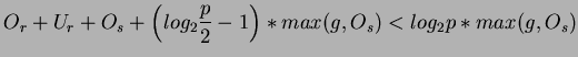
From this derivation, we conclude that if $(O_{r}+U_{r}+O_{s})<2g$ when $O_{s}<g$, or $(O_{r}+U_{r})<O_{s}$ when $g<O_{s}$, cost formula (2.8) is more appropriate to estimate the cost of this broadcast operation. Otherwise, use cost formula (2.9).