This parameter encapsulates all the costs involved in moving the data across the network, thus, it becomes an impracticable task to measure this parameter directly. For example, the physical network may stretch over the building, and therefore, direct signal analysis on two remote ends becomes impossible. A feasible approach to measure this movement cost is by indirect estimation. In this subsection, we first describe the indirect calculation that yields the approximation for the L values between two arbitrary cluster nodes, then we will describe the microbenchmark that portrays the L parameter for the whole cluster network.
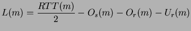
Recall that we can depict the total time for a m-byte packet to travel from the source node to its destination as
If we carry out a simple pingpong test, the measured roundtrip
time becomes
![]() . Since all other parameters
can be measured directly or indirectly, we can therefore deduce the
required L value by
. Since all other parameters
can be measured directly or indirectly, we can therefore deduce the
required L value by
Thus, equation (A.4) becomes an indirect measurement for the L parameter between two machines over a range of packet sizes.
However, showing the L value between two machines of the cluster
only delineates part of the cost, since the data are measured under
a competition-free condition. To capture the network performance,
our microbenchmark works up by generating multiple distinct pairs
of pingpong nodes, with nodes of each distinct pair lie across the
bisectional plane of the network. When all nodes start the pingpong
tests at the same time, this emulates multiple concurrent packets
flowing back-and-forth over the bisectional plane. Under this benchmark
setting, by varying the number of pingpong pairs, we obtain different
sets of L values. Then, the required bilinear function could
be obtained by applying multiple regression technique on these datasets.
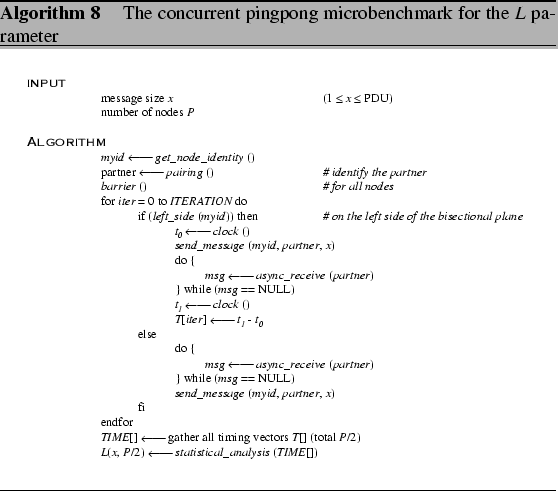
To summarize, Algorithm 8 presents the pseudocode for this
microbenchmark.
|
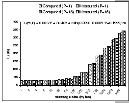
[(Cisco 2980G) - Comparison of calculated and measured L values on 2P=2 and 2P=32]
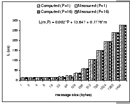 [(HN 8x4) - Comparison of calculated and measured L values on 2P=2 and 2P=32] [(HN 8x4) - Comparison of calculated and measured L values on 2P=2 and 2P=32]
[(HN 16x2) - Comparison of calculated and measured L values on 2P=2 and 2P=32]
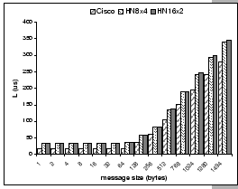
 [Comparison of three different configurations on a 32-node cluster] [Comparison of three different configurations on a 32-node cluster]
|