In this section, we are exploring the contention behavior of our lightweight reliable transmission protocol on different buffering architectures under the same traffic pattern - the many-to-one flow. The function of a reliable protocol in the communication system is for prevention of and/or recovery from any data loss. Most of the data loss situations in modern networks are caused by dropping of packets in the switches, which in turn are induced by the contention problem. We believe that with a better understanding on how buffering within switches affect the performance of the communication system, especially under heavy contention situation, more effective congestion avoidance schedules can be designed for the cluster domain.
Although this communication pattern induces the heaviest congestion on the network link(s), the congestion behavior of this traffic pattern is easier to comprehend than that of the many-to-many communication pattern. The obvious result of this many-to-one traffic is the congestion build-up at the outgoing port(s), to which directly or indirectly connected to the gather root (common sink) of this traffic pattern. As the outgoing link is over-subscribed, excessive packets must be buffered. If the congestion persists for a ``long'' duration, congestion loss will be the result. However, if the volume of the data bursts were within the storage capacity associated with this congested port, no packet would be loss. Therefore, the circumstance that induces packet loss under such a traffic pattern is the arrival of a large burst of data packets targeting to the same outgoing port within a close interval, and the volume of this burst overshoots the storage capacity as well as the drainage speed of the congested port. Moreover, on steady-state condition, the incoming and outgoing flows should become balance since data traffics are regulated by the flow-control protocol. This is commonly known as the "self-clocking" [51] effect of the flow-control protocol. Therefore, we deduce that bursts of data packets are only generated by the sources either at the start of the many-to-one traffic or after any packet loss incident.
In the beginning, all sources have a full window, so packets are injecting
into the network at full speed. Therefore, we observe that the volume
of the first burst of data packets is proportional to the flow control
window size (![]() ) and the number of concurrent senders (
) and the number of concurrent senders (![]() ).
If the buffering capacity (
).
If the buffering capacity (![]() ) of the bottleneck region
along the route of this flow is not large enough to accommodate this
burst, a "cluster of packets" is dropped. In this
study, we assume that all switches employ the drop-tail FIFO disciplinetypeset@protect
@@footnote
SF@gobble@opt
This is the most commonly used dropping discipline in commercial products.
[36] as the buffer management strategy; thus, when
the buffer is full, newcomers are discarded. Due to this dropping
discipline, packet losses are exhibiting some form of temporal correlation.
This is inferred from the following observations. First, if a packet
arrives at a congested port is dropped by the switch, packets from
different sources arriving to this bottleneck region in close apart
are likely to be lost too. Second, if a particular data stream loses
a packet, most of the subsequence packets originated from the same
sender within the same window session are likely to be lost too. The
implication of this packet loss behavior is that these sources will
receive the packet loss signals (negative acknowledgments or timeouts)
after sometime later but again in close apart. This triggers the error
recovery layer to recover from the loss and induces another burst
of data packets. Depends on the protocol used by the error recovery
layer, this phenomenon may continue to evolve and results in poor
network performance as the efficiency of the communication system
deteriorates significantly.
) of the bottleneck region
along the route of this flow is not large enough to accommodate this
burst, a "cluster of packets" is dropped. In this
study, we assume that all switches employ the drop-tail FIFO disciplinetypeset@protect
@@footnote
SF@gobble@opt
This is the most commonly used dropping discipline in commercial products.
[36] as the buffer management strategy; thus, when
the buffer is full, newcomers are discarded. Due to this dropping
discipline, packet losses are exhibiting some form of temporal correlation.
This is inferred from the following observations. First, if a packet
arrives at a congested port is dropped by the switch, packets from
different sources arriving to this bottleneck region in close apart
are likely to be lost too. Second, if a particular data stream loses
a packet, most of the subsequence packets originated from the same
sender within the same window session are likely to be lost too. The
implication of this packet loss behavior is that these sources will
receive the packet loss signals (negative acknowledgments or timeouts)
after sometime later but again in close apart. This triggers the error
recovery layer to recover from the loss and induces another burst
of data packets. Depends on the protocol used by the error recovery
layer, this phenomenon may continue to evolve and results in poor
network performance as the efficiency of the communication system
deteriorates significantly.
When analyzing the contention behavior of the many-to-one traffic in a cluster interconnect, two features should be considered. First, congestion loss only occurs when the first burst of data packets overruns the switch buffer. If the buffer capacity can tolerate the flooding, we would not see any congestion loss problem. Second, the reliable transmission protocol has significant impact on the available throughput especially when congestion loss occurs. Therefore, the overall congestion behavior with respect to the many-to-one flow would be a combined effect of the buffering mechanism and the reliable transmission protocol in use.
For a switched network, the buffering's ability to tolerate congestion is determined by three factors:
In this section, we are going to devise a simple empirical formula,
which predicts the performance observed by the end-user, when suffered
from contention loss on an input-buffered switch using the GBN scheme
described in previous section. Assumed that there are P data
sources and the many-to-one flow starting at time ![]() , where
all sources start sending their data packets more or less at the same
time. Initially, all sources have an open window of size
, where
all sources start sending their data packets more or less at the same
time. Initially, all sources have an open window of size ![]() (in unit of fixed-size packet), and they continually send out their
packets to the gather root. Congestion starts to build-up as we have
more than one active sender, so packets are buffered at the dedicated
memory associated to each ingress port - the input-buffered architecture.
As the buffer size is finite which is of
(in unit of fixed-size packet), and they continually send out their
packets to the gather root. Congestion starts to build-up as we have
more than one active sender, so packets are buffered at the dedicated
memory associated to each ingress port - the input-buffered architecture.
As the buffer size is finite which is of ![]() unit, thus,
at any given time
unit, thus,
at any given time ![]() , we observe that the queue size (
, we observe that the queue size (![]() )
must satisfy this constraint,
)
must satisfy this constraint,
![]() . Furthermore,
after the initial burst, all data flows should be regulated by the
gather root under normal circumstances. Therefore, we could see that
the congestion loss situation on the input-buffered architecture would
happen only if the initial burst were larger than the buffering capacity,
i.e. when
. Furthermore,
after the initial burst, all data flows should be regulated by the
gather root under normal circumstances. Therefore, we could see that
the congestion loss situation on the input-buffered architecture would
happen only if the initial burst were larger than the buffering capacity,
i.e. when
![]() . In other words, to avoid congestion
loss on the many-to-one data flow under an input-buffered switch,
one should have a window size (
. In other words, to avoid congestion
loss on the many-to-one data flow under an input-buffered switch,
one should have a window size (![]() ) which is smaller than
or equal to the input port buffering size (
) which is smaller than
or equal to the input port buffering size (![]() ).
).
|
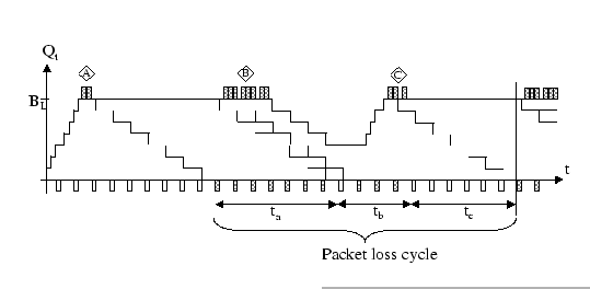
After the initial burst, as the departure rate of this buffering system
is slower than the input rate and the volume of the burst is larger
than the buffering capacity, packets at the end of the burst are dropped
(label A in Figure 4.2). However, the sender wouldn't detect
the loss until the first out-of-sequence packet reaches the gather
root (start of period ![]() ), and stimulates a packet loss
signal (Nack). As presented in Figure 4.1, the immediate response
of the sender to the reception of the Nack is to transit to the ReSend
state, and retransmits all outstanding packets (another burst of full
window packets). Then it waits at the Stall state until it receives
the first positive acknowledgement.
), and stimulates a packet loss
signal (Nack). As presented in Figure 4.1, the immediate response
of the sender to the reception of the Nack is to transit to the ReSend
state, and retransmits all outstanding packets (another burst of full
window packets). Then it waits at the Stall state until it receives
the first positive acknowledgement.
Under self-clocking principle, removal of one packet at the head of
the queue will induce the arrival of another packet to fill the space.
However, with an out-of-sequence packet, more than one data packets
are injected to the network which causes another period of congestion
loss (label B in Figure 4.2). For this burst, as there is
only one buffer space left in the queue, thus, only the first packet
can get a buffer slot. Since this is the expected packet that the
gather root is waiting for, this results in changing the sender from
the Stall state back to the normal state. In Figure 4.2,
we have labeled the period starting from the detection of the first
out-of-sequence packet to the time slot just before the reception
of the correct retransmitted packet be period ![]() . Within
this period, all packets received by the gather root are discarded
as they are out-of-sequence packets (the consequence of packet loss
at label A). Moreover, since the retransmission burst (label B) only
appears at the start of this period, and there is only limited space
left behind in the queue, most of those packets are dropped. The queue
size
. Within
this period, all packets received by the gather root are discarded
as they are out-of-sequence packets (the consequence of packet loss
at label A). Moreover, since the retransmission burst (label B) only
appears at the start of this period, and there is only limited space
left behind in the queue, most of those packets are dropped. The queue
size ![]() will gradually drop off as packets are continually
drained away without replacement.
will gradually drop off as packets are continually
drained away without replacement.
Although the sender transits from the Stall state back to the normal
state at the start of period ![]() , it immediately changes
back to the ReSend state after the gather root receives the next packet,
which is an out-of-sequence packet. Then another burst of packets
is generated by the sender, which starts to fill all buffer memory
again, and eventually induces another overflow situation (label C).
We depict the period
, it immediately changes
back to the ReSend state after the gather root receives the next packet,
which is an out-of-sequence packet. Then another burst of packets
is generated by the sender, which starts to fill all buffer memory
again, and eventually induces another overflow situation (label C).
We depict the period ![]() to be a period between the two transitions
of the sender from the Stall state back to the normal state. Like
period
to be a period between the two transitions
of the sender from the Stall state back to the normal state. Like
period ![]() , all packets except the first packet received
by the gather root in period
, all packets except the first packet received
by the gather root in period ![]() are out-of-sequence packets
(the consequence of packet loss at label B). Switching back to the
normal state marks the start of period
are out-of-sequence packets
(the consequence of packet loss at label B). Switching back to the
normal state marks the start of period ![]() . Within this period,
the gather root receives a sequence of in-order packets, which is
the outcome of the retransmission burst happened during period
. Within this period,
the gather root receives a sequence of in-order packets, which is
the outcome of the retransmission burst happened during period ![]() .
And period
.
And period ![]() ends with the gather root switches back to
the ReSend state when it detects an out-of-sequence packet, which
is the consequence of the overflow situation at the end of the retransmission
burst at label C.
ends with the gather root switches back to
the ReSend state when it detects an out-of-sequence packet, which
is the consequence of the overflow situation at the end of the retransmission
burst at label C.
When we carefully look at the evolution of the queue size as well
as the changes of packet statuses, we could find that the packet sequences
in periods ![]() to
to ![]() form a pattern that is recurred
over time. Thus, we could simplify our analysis by focusing on the
derivation of the throughput efficiency observed in this recurrent
cycle - the packet loss cycle. We define the throughput efficiency
(
form a pattern that is recurred
over time. Thus, we could simplify our analysis by focusing on the
derivation of the throughput efficiency observed in this recurrent
cycle - the packet loss cycle. We define the throughput efficiency
(![]() ) to be
) to be
where I denotes the average number of in-order packets
delivered to the gather root by this sender during a packet loss cycle,
and Õ be the average number of error packets received but originated
from this sender in the same period. To derive I and Õ, we
need to consider the three subintervals in the packet loss cycle and
count their corresponding number of good and error packets in each
period. We have seen that period ![]() is consisted of solely
out-of-sequence packets. The start of this period marks the first
error packet caused by the congestion loss at label A. Intuitively,
this error packet must move forward
is consisted of solely
out-of-sequence packets. The start of this period marks the first
error packet caused by the congestion loss at label A. Intuitively,
this error packet must move forward ![]() unit before it
gets to the head of the queue. When the gather root receives this
error packet, this causes the gather root to send back a Nack to the
sender, which results in filling up the last buffer space by a good
packet, and this good packet denotes the end of the period
unit before it
gets to the head of the queue. When the gather root receives this
error packet, this causes the gather root to send back a Nack to the
sender, which results in filling up the last buffer space by a good
packet, and this good packet denotes the end of the period ![]() .
Therefore, we deduce that within the
.
Therefore, we deduce that within the ![]() period, the gather
root receives
period, the gather
root receives ![]() units of error packets.
units of error packets.
Similarly, the error packets found in period ![]() are induced
by the retransmission burst at label B. As the expected arrival rate
of this burst is one packet per time slot, while the average departure
rate of this buffering system is one packet per P time slots,
we deduct that only
are induced
by the retransmission burst at label B. As the expected arrival rate
of this burst is one packet per time slot, while the average departure
rate of this buffering system is one packet per P time slots,
we deduct that only
![]() packets could be buffered
when they arrive to the input FIFO queue. However, all of these buffered
packets are out-of-sequence packets. After this retransmission burst
(label B), the sender transits to the Stall state. No more packets
are sent to the queue until it changes back to the normal state at
the start of period
packets could be buffered
when they arrive to the input FIFO queue. However, all of these buffered
packets are out-of-sequence packets. After this retransmission burst
(label B), the sender transits to the Stall state. No more packets
are sent to the queue until it changes back to the normal state at
the start of period ![]() , then the sender injects another
packet to the queue which again is an out-of-sequence packet. Therefore,
we could see that the expected number of good packets received by
the gather root during period
, then the sender injects another
packet to the queue which again is an out-of-sequence packet. Therefore,
we could see that the expected number of good packets received by
the gather root during period ![]() is one packet, and the
expected number of error packets received in this period is
is one packet, and the
expected number of error packets received in this period is
![]() packets. Based on the same principle, we estimate the amount of good
packets buffered within period
packets. Based on the same principle, we estimate the amount of good
packets buffered within period ![]() . Before the retransmission
burst arrived to the FIFO queue at the start of period
. Before the retransmission
burst arrived to the FIFO queue at the start of period ![]() ,
there are
,
there are
![]() error packets in the queue. So
we would expect to have
error packets in the queue. So
we would expect to have
 buffer
space to accommodate those in-order packets before the buffer overflow
situation happens again, and this becomes the amount of good packets
received in period
buffer
space to accommodate those in-order packets before the buffer overflow
situation happens again, and this becomes the amount of good packets
received in period ![]() . Thus, the throughput efficiency observed
in a packet loss cycle becomes
. Thus, the throughput efficiency observed
in a packet loss cycle becomes
Although ![]() is derived by observing the dynamic behavior
within a single input FIFO queue, if we assume that the same situation
happens to all input FIFO queues and each sender gets a fair share
(i.e.
is derived by observing the dynamic behavior
within a single input FIFO queue, if we assume that the same situation
happens to all input FIFO queues and each sender gets a fair share
(i.e.
![]() ) of the available bandwidth, then the expected
throughput efficiency observed on this many-to-one flow should be
) of the available bandwidth, then the expected
throughput efficiency observed on this many-to-one flow should be
In conclusion, from formula (4.2), we observe that with the
congestion loss problem, the sustained throughput of this many-to-one
flow would be less than 50% of the available bandwidth, since the
denominator is at least twice as large as the numerator. As congestion
loss problem only happens when
![]() , thus we just need
to consider the effect of
, thus we just need
to consider the effect of ![]() only. From the formula, we
observe that the
only. From the formula, we
observe that the ![]() factor has a negative linear relation
with the throughput efficiency, such that if we increase
factor has a negative linear relation
with the throughput efficiency, such that if we increase ![]() ,
we would expect to have a decrease in the sustained throughput. As
for the factor
,
we would expect to have a decrease in the sustained throughput. As
for the factor ![]() , it seems to have insignificant effect on
the final throughput.
, it seems to have insignificant effect on
the final throughput.
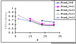
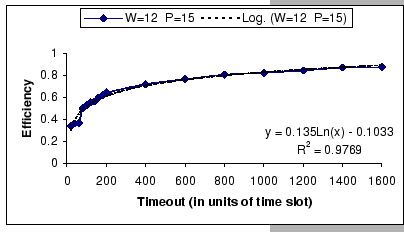
We validate
![]() by using measurement data obtained
from our experimental cluster platform. We use a cluster with 24 high-end
PCs (PIII 733) connected by the IBM 8275-326 Fast Ethernet switch,
which is revealed as an input-buffered architecture with
by using measurement data obtained
from our experimental cluster platform. We use a cluster with 24 high-end
PCs (PIII 733) connected by the IBM 8275-326 Fast Ethernet switch,
which is revealed as an input-buffered architecture with ![]() units per input port (Appendix A). To drive the Fast Ethernet
network, we use the Directed Point (DP) low-latency communication
system and implement the described Go-Back-N scheme to support reliability
on top of DP. We have shown in Chapter 3 that with such a
high-end cluster, the performance bottleneck falls on the network
component.
units per input port (Appendix A). To drive the Fast Ethernet
network, we use the Directed Point (DP) low-latency communication
system and implement the described Go-Back-N scheme to support reliability
on top of DP. We have shown in Chapter 3 that with such a
high-end cluster, the performance bottleneck falls on the network
component.
To simulate the many-to-one data flow under steady state streaming,
we gathered all performance data by running the Gather collective
operation with ![]() processes and each process sends out 30000
full size data packets to the gather root, e.g. for
processes and each process sends out 30000
full size data packets to the gather root, e.g. for ![]() , the
total message length received by the gather root is approximately
640MBtypeset@protect
@@footnote
SF@gobble@opt
The size of the received message is beyond the memory capacity of
a single cluster node, which only has 128 MB of primary memory. To
avoid paging overheads that affect the final throughput, all incoming
data to the gather root are discarded immediately after protocol checking,
thus without copying from the staging buffer to the user-space buffer.
This avoids the need to create such a large receive buffer, and hence,
avoids the paging overhead.
. To induce the congestion loss problem, we started the experiments
with
, the
total message length received by the gather root is approximately
640MBtypeset@protect
@@footnote
SF@gobble@opt
The size of the received message is beyond the memory capacity of
a single cluster node, which only has 128 MB of primary memory. To
avoid paging overheads that affect the final throughput, all incoming
data to the gather root are discarded immediately after protocol checking,
thus without copying from the staging buffer to the user-space buffer.
This avoids the need to create such a large receive buffer, and hence,
avoids the paging overhead.
. To induce the congestion loss problem, we started the experiments
with
![]() for various
for various ![]() , P
and timeout (TO) combinations, and observe their effects on the final
performance. To simplify our analysis, we assume that the timeout
value is set to a sufficient large value to avoid false retransmissiontypeset@protect
@@footnote
SF@gobble@opt
The setting of timeout value is depended on the available network
information. As this protocol is designed for communications on an
enclosed network with negligible transmission error, we can make use
of the
, P
and timeout (TO) combinations, and observe their effects on the final
performance. To simplify our analysis, we assume that the timeout
value is set to a sufficient large value to avoid false retransmissiontypeset@protect
@@footnote
SF@gobble@opt
The setting of timeout value is depended on the available network
information. As this protocol is designed for communications on an
enclosed network with negligible transmission error, we can make use
of the ![]() ,
, ![]() and
and ![]() parameters to estimate
the timeout setting, instead of using the round-trip estimation.
. Each test is conducted with P senders send out their messages ``continuously''
to the sole receiver and we measured how long would it take for all
processes to complete this collective operation. By dividing the theoretical
performance of the gather operation with the measured result, we calculate
the throughput efficiency of this gather operation under congestion
loss problem.
parameters to estimate
the timeout setting, instead of using the round-trip estimation.
. Each test is conducted with P senders send out their messages ``continuously''
to the sole receiver and we measured how long would it take for all
processes to complete this collective operation. By dividing the theoretical
performance of the gather operation with the measured result, we calculate
the throughput efficiency of this gather operation under congestion
loss problem.
|
[our GBN - Timeout = 1000]
 [simple GBN - Timeout = 1000] [simple GBN - Timeout = 1000]
[our GBN - Timeout = 2000]
 [simple GBN - Timeout = 2000] [simple GBN - Timeout = 2000]
[our GBN - Timeout = 2000]
 [simple GBN - Timeout = 2000] [simple GBN - Timeout = 2000]
[our GBN - P = 15]
 [simple GBN - P = 15] [simple GBN - P = 15]
|
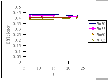
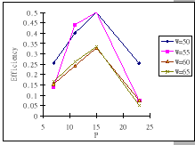
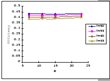
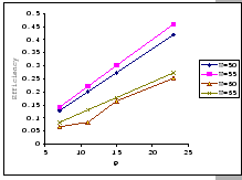
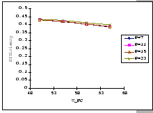
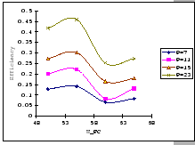
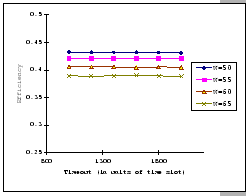
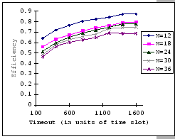
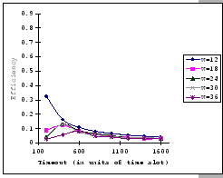
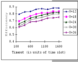
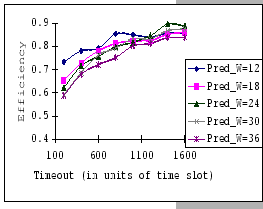
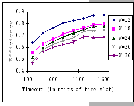
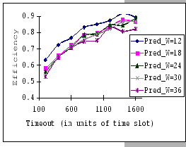
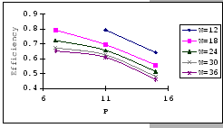
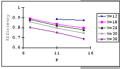
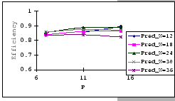
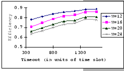
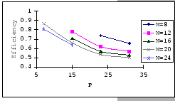
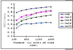
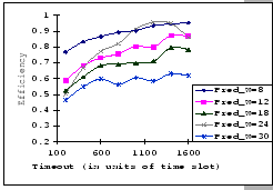
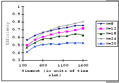
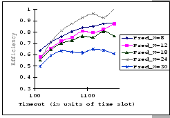
The first set of experimental results is presented in Figure 4.3.
In this figure, we are comparing the throughput efficiency (
![]() )
of our GBN scheme and a simple GBN scheme under the above experimental
settings on an input-buffered switch. The simple GBN scheme is the
classical version of the GBN scheme which does not have the fast retransmission
mechanism. Therefore, whenever the receiver receives an out-of-sequence
packet, it simply drops it and waits for the timeout retransmission.
In general, we see that the performance of our GBN scheme is better
than the simple GBN scheme, except on a few data points. Particularly,
our GBN scheme is quite insensitive to the number of senders and the
timeout parameter (Figure 4.3(a)(c)(g)), while the
simple GBN scheme varies substantially with different P,
)
of our GBN scheme and a simple GBN scheme under the above experimental
settings on an input-buffered switch. The simple GBN scheme is the
classical version of the GBN scheme which does not have the fast retransmission
mechanism. Therefore, whenever the receiver receives an out-of-sequence
packet, it simply drops it and waits for the timeout retransmission.
In general, we see that the performance of our GBN scheme is better
than the simple GBN scheme, except on a few data points. Particularly,
our GBN scheme is quite insensitive to the number of senders and the
timeout parameter (Figure 4.3(a)(c)(g)), while the
simple GBN scheme varies substantially with different P, ![]() and timeout parameters (Figure 4.3(b)(d)(f)(h)).
With the simple GBN scheme, we observe that the timeout value is closely
related to the number of senders (Figure 4.3(b)(d)).
Such that with each P value, there is a specific timeout setting that
fits it most, otherwise, the performance deteriorates considerably
(Figure 4.3(h)). Another interesting observation
on Figure 4.3 is that the achieved maximum throughput
efficiency is no better than 50% of the available bandwidth on both
GBN measurements.
and timeout parameters (Figure 4.3(b)(d)(f)(h)).
With the simple GBN scheme, we observe that the timeout value is closely
related to the number of senders (Figure 4.3(b)(d)).
Such that with each P value, there is a specific timeout setting that
fits it most, otherwise, the performance deteriorates considerably
(Figure 4.3(h)). Another interesting observation
on Figure 4.3 is that the achieved maximum throughput
efficiency is no better than 50% of the available bandwidth on both
GBN measurements.
|
[ Measured - Timeout=2000]
 [ Predicted -Timeout=2000] [ Predicted -Timeout=2000]
[ Measured - Timeout=2000]
 [ Predicted - Timeout=2000] [ Predicted - Timeout=2000]
[ Measured - P=15]
 [Predicted - P=15] [Predicted - P=15]
|
We have shown that with an input-buffered architecture, we lose more than 50% of the theoretical performance under congestion loss problem. In this section, we switch our analysis to the congestion dynamic happened on the output-buffered architecture under the same GBN ARQ scheme. Then based on these analytical studies, we compare on the performance differences between different buffering architectures.
With the output-buffered architecture, packets start to accumulate
in the buffers associated to the egress port that leads to the gather
root. As we assume that the buffer size is finite, at any given time
![]() , we observe that the queue size (
, we observe that the queue size (![]() ) must satisfy
this constraint,
) must satisfy
this constraint,
![]() . From this observation,
we conclude that the congestion loss situation would happen on this
architecture if and only if we have an initial burst of data packets
which is larger than
. From this observation,
we conclude that the congestion loss situation would happen on this
architecture if and only if we have an initial burst of data packets
which is larger than ![]() , such that, when
, such that, when
![]() .
As compare to input-buffered architecture with the same per port buffering
capacity and under the same number of sources, the output-buffered
architecture is more sensitive to the congestion loss problem under
the many-to-one flow.
.
As compare to input-buffered architecture with the same per port buffering
capacity and under the same number of sources, the output-buffered
architecture is more sensitive to the congestion loss problem under
the many-to-one flow.
To study the steady state contention behavior, we assume that the
communication event starts with
![]() and all sources
have unlimited amount of data to send. We also assume that our switched
network adopts the drop tail discipline, and packets that arrive at
a full buffer are dropped unconditionally. This dropping policy induces
some form of temporally correlation amongst the senders, which results
in creating wave of retransmission bursts. Under such scenario, some
senders fall through to Stall state as their first packets cannot
find an empty slot in the output queue, and thus, get into hibernation
(i.e. remain inactive until retransmission timer expire). Some senders
may alternate between cycles of Pack
and all sources
have unlimited amount of data to send. We also assume that our switched
network adopts the drop tail discipline, and packets that arrive at
a full buffer are dropped unconditionally. This dropping policy induces
some form of temporally correlation amongst the senders, which results
in creating wave of retransmission bursts. Under such scenario, some
senders fall through to Stall state as their first packets cannot
find an empty slot in the output queue, and thus, get into hibernation
(i.e. remain inactive until retransmission timer expire). Some senders
may alternate between cycles of Pack
![]() Nack events
and eventually get into hibernation too. Only limited number of senders
could get through this contention period and remain active until those
slumbering senders receive their timeout signals and start another
cycle of congestion. Therefore, if we collect the activity profile
of a particular sender, we would see that its activities are cycling
between Pack, Nack and Timeout events. Figure 4.5 shows a
sample trace of the sender's activities which corresponds to such
an arbitrary sequence of state transitions over time
Nack events
and eventually get into hibernation too. Only limited number of senders
could get through this contention period and remain active until those
slumbering senders receive their timeout signals and start another
cycle of congestion. Therefore, if we collect the activity profile
of a particular sender, we would see that its activities are cycling
between Pack, Nack and Timeout events. Figure 4.5 shows a
sample trace of the sender's activities which corresponds to such
an arbitrary sequence of state transitions over time
|
(Legend:
|
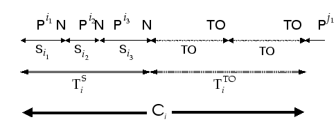
Based on the above observations, we model the congestion behavior of our reliable protocol in terms of activity cycles of the sender, with each cycle is characterized by some recurrent patterns which we believe, are statistical independent but are probabilistic replicas of one another. A sample cycle is given in Figure 4.6 which is an abstract representation of the sample trace shown in Figure 4.5.
|
Now we are going to derive an analytical model that captures the throughput
efficiency observed by a particular sender under this buffering architecture.
Let
![]() denotes the duration of a sequence of timeout
events and
denotes the duration of a sequence of timeout
events and ![]() be the time interval between two consecutive
timeout sequences. When adding up these two intervals, we have
be the time interval between two consecutive
timeout sequences. When adding up these two intervals, we have
![]() ,
which becomes the elapsed time of a particular activity cycle. We
also define
,
which becomes the elapsed time of a particular activity cycle. We
also define ![]() be the number of in-order packets received
by the gather root with respect to this sender during this
be the number of in-order packets received
by the gather root with respect to this sender during this ![]() interval. By viewing
interval. By viewing
![]() as
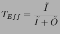
a stochastic sequence of random variables, we define the throughput
efficiency be
as
a stochastic sequence of random variables, we define the throughput
efficiency be
![$\displaystyle T_{Eff}=\frac{E[U]}{\frac{E[C]}{g_{r}}}=\frac{E[U]*g_{r}}{E[C]}$](img191.png)
where E[U] denotes the expected number of packets accepted
by the gather root in one activity cycle and E[C] be the expected
duration of one activity cycle. Without having packet loss, we expect
that the gather root can handle one packet per ![]() time units,
thus, the maximum number of packets that a the gather root can handle
during E[C] time units is
time units,
thus, the maximum number of packets that a the gather root can handle
during E[C] time units is
![]() packets.
packets.
To derive E[U], we have to estimate the total number of Pack responses
received within those
![]() sequences. Let
sequences. Let ![]() be the number of
be the number of
![]() sequences in the interval
sequences in the interval ![]() .
For the k-th
.
For the k-th
![]() sequence, we define
sequence, we define ![]() to be the number of Pack responses received in that period,
to be the number of Pack responses received in that period, ![]() to be the duration of that period. Assume if the number of Pack responses
received in one
to be the duration of that period. Assume if the number of Pack responses
received in one
![]() sequence is statistically independent
to the number of Pack responses in another
sequence is statistically independent
to the number of Pack responses in another
![]() sequence,
then we can view
sequence,
then we can view
![]() as a sequence of
independent and identically distributed (i.i.d) random variables.
The same assumption can be applied to
as a sequence of
independent and identically distributed (i.i.d) random variables.
The same assumption can be applied to ![]() and
and ![]() .
Now we have
.
Now we have
![$\displaystyle U_{i}=\sum _{k=1}^{y_{i}}x_{i_{k}}\: \: \Rightarrow \: \: E[U]=E\left[ \sum ^{y_{i}}_{k=1}x_{i_{k}}\right] \: \: \Rightarrow \: \: E[U]=E[y]*E[x]$](img197.png)
![$\displaystyle T_{i}^{S}=\sum ^{y_{i}}_{k=1}S_{i_{k}}\: \: \Rightarrow \: \: E[T...
... \sum ^{y_{i}}_{k=1}S_{i_{k}}\right] \: \: \Rightarrow \: \: E[T^{S}]=E[y]*E[S]$](img198.png)
As for deriving E[C], let ![]() be the number of timeout
periods in the interval
be the number of timeout
periods in the interval
![]() and since the duration of
each timeout period is fixed, we have
and since the duration of
each timeout period is fixed, we have
Assume that the number of timeout periods in each activity cycle is also an i.i.d random variable, then we have
and thus,
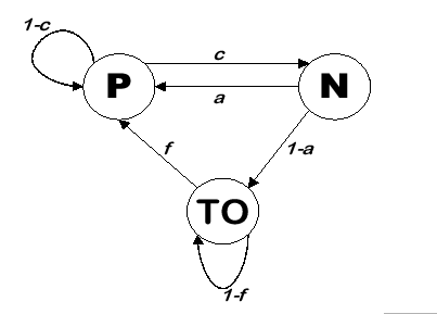
To derive E[y], E[x] and E[m], we make use of concepts from discrete-time Markov chain model [50] to model the activity profile of a sender. A 3-state Markov chain model (see Figure 4.7) is constructed which represents the three different events happened in a sender profile, they are P - Pack, N - Nack and TO - timeout events. With reference to the state transition diagram (Figure 4.1) of our GBN protocol, a Pack event means working in normal state or transit to normal state, a Nack event means transit to the ReSend state (fast retransmission), and the TO event means slumbering in the Stall state but being waked up by the timeout signal. However, transition from one event status to another means the detection of or recovery from some loss events. Therefore, the transition probabilities between certain events are directly related to the loss probabilities on the congested path.
Hence, we define the stochastic process in which this 3-state loss
model is based on as,
![]() = the type of events delivered
to the sender at the time of receiving the
= the type of events delivered
to the sender at the time of receiving the ![]() event with
a finite state space,
event with
a finite state space,
![]() , and the corresponding
transition probability matrix is
, and the corresponding
transition probability matrix is
![$\displaystyle \left[ \begin{array}{ccc}
1-c & c & 0\\
a & 0 & 1-a\\
f & 0 & 1-f
\end{array}\right] ,$](img206.png)
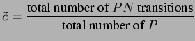
Now we first derive E[x]. Given our loss model and the assumption
of being a stationarytypeset@protect
@@footnote
SF@gobble@opt
The probability of going from one state to another is independent
of the time at which the step is being made [50].
discrete-time Markov chain, the probability that
![]() is equal to the probability that there appears to have
is equal to the probability that there appears to have ![]() P
events before a PN transition occurs. Thus,
P
events before a PN transition occurs. Thus,
Finally, to derive an expression for E[S], we look into the time scale of a particular
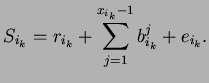
![$\displaystyle E[S]=E[r]+E\left[ \sum ^{x_{i_{k}}-1}_{j=1}b_{i_{k}}^{j}\right] +E[e]$](img233.png)
From Figure 4.8, we see that ![]() is the time
lapsed between a Nack event and a Pack event. When a sender receives
an Nack event, it responses by re-sending all outstanding packets,
and we would expect that the next Pack event is triggered by the reception
of the first packet from this ReSend burst. Therefore the elapsed
time between this Nack/Pack pair depends on the current queue size
(
is the time
lapsed between a Nack event and a Pack event. When a sender receives
an Nack event, it responses by re-sending all outstanding packets,
and we would expect that the next Pack event is triggered by the reception
of the first packet from this ReSend burst. Therefore the elapsed
time between this Nack/Pack pair depends on the current queue size
(![]() ) as the first packet of the ReSend burst needs to move
forward to the head of the queue before a Pack event is generated.
Since
) as the first packet of the ReSend burst needs to move
forward to the head of the queue before a Pack event is generated.
Since ![]() is bounded by
is bounded by ![]() , and under steady state
condition on the many-to-one flow, the buffer queue should operate
under almost full condition. Thus, we have
, and under steady state
condition on the many-to-one flow, the buffer queue should operate
under almost full condition. Thus, we have
![$\displaystyle E[b]=E[A]*g_{r}=\frac{B_{L}*g_{r}}{W_{FC}}.$](img240.png)
We follow the same logic to deduce ![]() Remember that a Pack
is sent to a sender only when the gather root receives an in-order
packet from that sender. So the inter-arrival time (
Remember that a Pack
is sent to a sender only when the gather root receives an in-order
packet from that sender. So the inter-arrival time (![]() ) between
Pack events has a direct relationship with the elapsed time between
consecutive packets from the same sender. To determine
) between
Pack events has a direct relationship with the elapsed time between
consecutive packets from the same sender. To determine ![]() ,
we have to estimate how many packets from this sender are lost before
the gather root detects this loss problem. If we consider the loss
is uniformly distributed between 1 and
,
we have to estimate how many packets from this sender are lost before
the gather root detects this loss problem. If we consider the loss
is uniformly distributed between 1 and ![]() , then on average,
we would expect to have
, then on average,
we would expect to have
![]() lost packets before
the gather root detects the loss situation. Since each consecutive
packet is separated by
lost packets before
the gather root detects the loss situation. Since each consecutive
packet is separated by ![]() time units,
time units, ![]() becomes
becomes
![$\displaystyle E[e]=\frac{W_{FC}-1}{2}*E[b]=\frac{(W_{FC}-1)*B_{L}*g_{r}}{2W_{FC}}.$](img245.png)
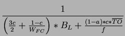
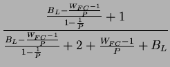
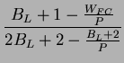
The above empirical equation (4.9) for predicting the throughput
efficiency on the output-buffered architecture is formulated in terms
of 3 transition probabilities - a, c and f. From
the formula, we observe that transition probability c has a
significant role on the final performance, such that if we can find
some way to minimize c, the higher throughput we get. To utilize
this equation, we need to provide some methods to determine these
probabilities. However, we cannot identify a clean association between
our target performance parameters (![]() ,
, ![]() ,
, ![]() & TO) and those transition probabilities. Consequently, we
have to rely on some inferential approach [50]
to statistically estimate these transition probabilities, which is
commonly used in other performance studies [119,74,112,63].
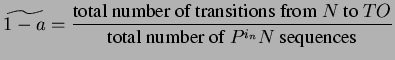
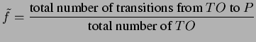
In particular, we look at the information gathered from a sample trace
and use this information to estimate on the transition probabilities.
For examples, in our case, we have
& TO) and those transition probabilities. Consequently, we
have to rely on some inferential approach [50]
to statistically estimate these transition probabilities, which is
commonly used in other performance studies [119,74,112,63].
In particular, we look at the information gathered from a sample trace
and use this information to estimate on the transition probabilities.
For examples, in our case, we have
A series of experiments are conducted to validate the above empirical
formula. For all of these tests, the same cluster that we have used
in Subsection 4.3.2.1 is used, however, the number
of cluster nodes involved depends on the configuration of the switch
or at most 32 nodes. Furthermore, the same GBN reliable transmission
protocol and the DP package are used. The first set of experiments
is conducted with this cluster interconnected by the 16-port IBM 8275-416
Ethernet switch. Under our benchmark tests, this switch is revealed
to have an output-buffered architecture with ![]() units
per output port. As this switch can only support 16 full 100 Mb/s
connections, we use a cluster size of 16 nodes to conduct all tests.
The second set of experiments are conducted by interconnecting this
cluster with the Cisco Catalyst 2980G Ethernet switch, which has 80
Fast Ethernet ports and 2 Gigabit Ethernet ports. By applying our
benchmark tests on this switch, we uncover that the switch internal
is adopting an output-buffered allocation scheme on a shared memory
architecturetypeset@protect
@@footnote
SF@gobble@opt
On the supporting document of this switch [99], Cisco
claims that this switch has a low-latency, centralized, shared memory
switching fabric architecture.
(with
units
per output port. As this switch can only support 16 full 100 Mb/s
connections, we use a cluster size of 16 nodes to conduct all tests.
The second set of experiments are conducted by interconnecting this
cluster with the Cisco Catalyst 2980G Ethernet switch, which has 80
Fast Ethernet ports and 2 Gigabit Ethernet ports. By applying our
benchmark tests on this switch, we uncover that the switch internal
is adopting an output-buffered allocation scheme on a shared memory
architecturetypeset@protect
@@footnote
SF@gobble@opt
On the supporting document of this switch [99], Cisco
claims that this switch has a low-latency, centralized, shared memory
switching fabric architecture.
(with ![]() units per output port). We only connect 32
cluster nodes to this switch as this is the maximum size we have for
this homogeneous cluster.
units per output port). We only connect 32
cluster nodes to this switch as this is the maximum size we have for
this homogeneous cluster.
We employ a similar testing methodology as appeared in Subsection
4.3.2.1 on each platform, however, to induce the congestion
loss problem, we have a different window sizing constraint, that is
![]() . Since the two switching platforms have different
buffering capacity and supported port number, thus the extent of varying
the
. Since the two switching platforms have different
buffering capacity and supported port number, thus the extent of varying
the ![]() and
and ![]() parameters are different too. In order
to apply our empirical formula (Eq. 4.9), we collect activity
traces from those processes during the tests. We obtain the measured
performance on different parameter settings (different combinations
of
parameters are different too. In order
to apply our empirical formula (Eq. 4.9), we collect activity
traces from those processes during the tests. We obtain the measured
performance on different parameter settings (different combinations
of ![]() ,
, ![]() and
and ![]() ) by running the same tests
for 30 iterations and take the average timing as the result measurement.
To minimize the required runtime memory to store the activity traces,
only the activity traces of all senders on the last iteration are
returned. Then the corresponding transition probabilities are calculated
for each sender, and finally, the mean values from all the senders
are taken as the transition probabilities for this particular parameter
set. Table 4.1 displays a sample set of data collected
from the IBM 8275-416 platform by this method.
) by running the same tests
for 30 iterations and take the average timing as the result measurement.
To minimize the required runtime memory to store the activity traces,
only the activity traces of all senders on the last iteration are
returned. Then the corresponding transition probabilities are calculated
for each sender, and finally, the mean values from all the senders
are taken as the transition probabilities for this particular parameter
set. Table 4.1 displays a sample set of data collected
from the IBM 8275-416 platform by this method.
|
|
[our GBN - Timeout = 1000]
 [simple GBN - Timeout = 1000] [simple GBN - Timeout = 1000]
[our GBN - Timeout = 1000]
 [simple GBN - Timeout = 1000] [simple GBN - Timeout = 1000]
[our GBN - P = 15]
 [simple GBN - P = 15] [simple GBN - P = 15]
|
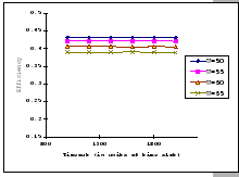
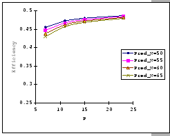
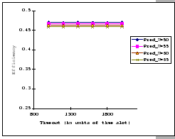
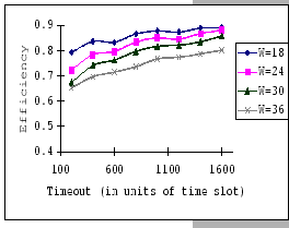
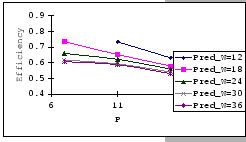
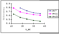
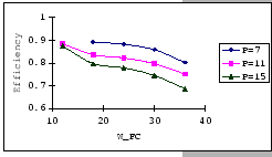
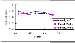
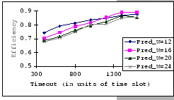
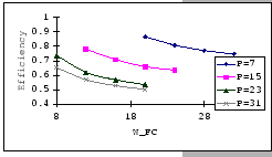
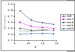
In Figures 4.10 and 4.11, we have the comparisons
of the measured and predicted performance of our GBN scheme on the
IBM 8275-416 platform for various parameter sets. In general, the
empirical formula (Eq. 4.10) correctly reflects the macroscopic
behavior of our GBN reliable transmission protocol on the output-buffered
architecture. Specifically, both the measured and predicted results
(Figure 4.10) show that having a larger TO setting
improves the throughput efficiency. This behavior is a result of the
addition of the fast retransmission mechanism, which randomly selects
a few senders to continue and denies the rest. Besides the TO
parameter, we also observe that both the ![]() and
and ![]() parameters are inversely related to the throughput efficiency.
parameters are inversely related to the throughput efficiency.
|
[Measured - P=7]
 [Predicted - P=7] [Predicted - P=7]
[Measured - P=11]
 [Predicted - P=11] [Predicted - P=11]
[Measured - P=15]
 [Predicted - P=15] [Predicted - P=15]
|
|
[Measured - Timeout=200]
 [Predicted - Timeout=200] [Predicted - Timeout=200]
[Measured - Timeout=200]
 [Predicted - Timeout=200] [Predicted - Timeout=200]
[Measured - Timeout=1600]
 [Predicted - Timeout=1600] [Predicted - Timeout=1600]
[Measured - Timeout=1600]
 [Predicted - Timeout=1600] [Predicted - Timeout=1600]
|
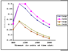
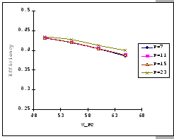
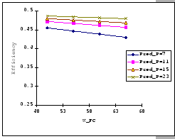
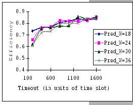
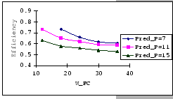
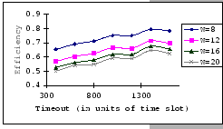
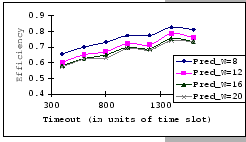
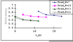
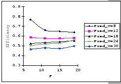
On the other hand, observing from the results shown in Table 4.1
and Figure 4.11, we find that the accuracy of our predictions
is deteriorating along with the increase in ![]() ,
, ![]() and
and ![]() , albeit the low error rate (the 95% confidence level
of the prediction error falls on
, albeit the low error rate (the 95% confidence level
of the prediction error falls on
![]() ). When the timeout
setting is small (subgraphs (a),(b),(c)&(d) of Figure 4.11),
we clearly see that our empirical formula correctly reflects the relationships
between
). When the timeout
setting is small (subgraphs (a),(b),(c)&(d) of Figure 4.11),
we clearly see that our empirical formula correctly reflects the relationships
between ![]() ,
, ![]() &
&
![]() , but when
the timeout setting is large, the relationships become unclear. This
is because, when look into the data shown in Table 4.1,
our empirical formula tends to over-estimate the improvement made
by the increase in timeout parameter.
, but when
the timeout setting is large, the relationships become unclear. This
is because, when look into the data shown in Table 4.1,
our empirical formula tends to over-estimate the improvement made
by the increase in timeout parameter.
|
[Measured - P=15]
 [Predicted - P=15] [Predicted - P=15]
[Measured - P=31]
 [Predicted - P=31] [Predicted - P=31]
[Measured - Timeout=400]
 [Predicted - Timeout=400] [Predicted - Timeout=400]
[Measured - Timeout=400]
 [Predicted - Timeout=400] [Predicted - Timeout=400]
|
|
|
In previous subsections, we have examined on the performance behavior of two buffering architectures under heavy congestion loss. Regards to the buffering architectures, another commonly used buffering scheme should also be considered - the shared-buffered [110] or common output-buffered architecture [42]. This scheme makes use of dynamic buffer allocation from a common pool of buffers, and therefore each output port virtually has a larger buffer storage. The main advantages of this scheme as compared to output-buffered architecture are (1) the higher buffer utilization can be achieved and (2) a smaller total buffering capacity is required. However, to avoid unfair utilization, most implementations set up an upper limit on each output port. Due to the architectural similarity between the shared-buffered and the output-buffered schemes, we consider that the above analytical study on the output-buffered scheme is directly applicable to the shared-buffered architecture.
We have two models that describe the congestion behavior of our communication
system under different buffering architectures; however, one can show
that the 3-state Markov chain model can be used to derive the input-buffered
case, if we view the input-buffered case as a special case of this
Markov chain model, where ![]() &
&
![]() .
Although using stochastic process to model system dynamic is a powerful
technique, it has some known limitations. For some cases, to capture
real world phenomena but still keeping the model equation tractable,
one has to rely on some known and well-behaved statistical or probabilistic
models. Then, the question becomes how close are these assumptions
matched with the reality? Besides, we may find that on some cases,
there exists no general probability model that suits for our needs.
Then one has to collect information from the running system, or if
a system does not exist, collect from the simulator. Therefore, in
all cases, analysts are required to have statistical expertise. Depending
on the techniques used, these skills are usually not common to the
parallel programmers [116]. Furthermore, of our study on
the output-buffered architecture, we are using the second method to
derive those transition probabilities. Although the prediction results
are within acceptable accuracy, we believe that the information revealed
by the empirical equation (4.10) for output-buffered is
not as expressive as that by the empirical equation (4.3)
for input-buffered. For example, one can directly estimate the effect
of varying the
.
Although using stochastic process to model system dynamic is a powerful
technique, it has some known limitations. For some cases, to capture
real world phenomena but still keeping the model equation tractable,
one has to rely on some known and well-behaved statistical or probabilistic
models. Then, the question becomes how close are these assumptions
matched with the reality? Besides, we may find that on some cases,
there exists no general probability model that suits for our needs.
Then one has to collect information from the running system, or if
a system does not exist, collect from the simulator. Therefore, in
all cases, analysts are required to have statistical expertise. Depending
on the techniques used, these skills are usually not common to the
parallel programmers [116]. Furthermore, of our study on
the output-buffered architecture, we are using the second method to
derive those transition probabilities. Although the prediction results
are within acceptable accuracy, we believe that the information revealed
by the empirical equation (4.10) for output-buffered is
not as expressive as that by the empirical equation (4.3)
for input-buffered. For example, one can directly estimate the effect
of varying the ![]() parameter from equation (4.3),
while equation (4.10) only shows part of the picture as
we cannot take hold of the relationship between
parameter from equation (4.3),
while equation (4.10) only shows part of the picture as
we cannot take hold of the relationship between ![]() and
those transition probabilities.
and
those transition probabilities.
The primary objective of this study is to explore the relationship between buffering architecture and congestion behavior, and through the analysis, we could devise better strategies in handling the contention problem. Although our studies are based on the many-to-one pattern with a single switched network, we believe that our findings can be extended to capture the congestion behavior of different network configurations and communication scenarios. In short summary, here are what we have observed from our analytical studies and previous experiments:
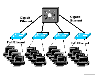
For the first set of tests on the hierarchical network, we show that
the congestion behavior of the output-buffered case can be used to
explain on the congestion behavior of an input-buffered port, which
happens to be the bridging port between the two Ethernet technologies.
Using the same cluster as in previous experiments, we connect 10 cluster
nodes to one IBM 8275-326 switch and there are total three such subnets
in this setup. Each IBM 8275-326 switch is connected to a Gigabit
Ethernet switch - the Alcatel PowerRail 2200 (PR2200), through a Gigabit
uplink port. With this configuration, in theory, we have full-connectivity
for all 30 machines. After running our benchmark tests, we find that
this Gigabit uplink port has an input-buffered architecture with ![]() units (which matches with buffer size of other FE ports). However,
we also uncover a serious problem of this uplink port. Although it
is capable to sustain ten full FE streams on the upstream flowtypeset@protect
@@footnote
SF@gobble@opt
Upstream - movement of data from the low-level to upper-level of the
hierarchy; while downstream is just the reverse.
, it could only manage to sustain at most seven full FE streams on
the downstream flow without packet loss. More discussion will be given
later in this subsection. As for the PR2200 GE switch, our benchmark
tests show that it has a shared-buffered architecture with
units (which matches with buffer size of other FE ports). However,
we also uncover a serious problem of this uplink port. Although it
is capable to sustain ten full FE streams on the upstream flowtypeset@protect
@@footnote
SF@gobble@opt
Upstream - movement of data from the low-level to upper-level of the
hierarchy; while downstream is just the reverse.
, it could only manage to sustain at most seven full FE streams on
the downstream flow without packet loss. More discussion will be given
later in this subsection. As for the PR2200 GE switch, our benchmark
tests show that it has a shared-buffered architecture with ![]() units.
units.
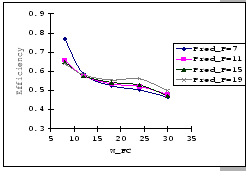
|
|
[Measured - P=7]
 [Predicted - P=7] [Predicted - P=7]
[Measured - P=19]
 [Predicted - P=19] [Predicted - P=19]
[Measure - Timeout=200]
 [Predicted - Timeout=200] [Predicted - Timeout=200]
[Measured - Timeout=200]
 [Predicted - P=200] [Predicted - P=200]
|
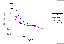
In the previous experiments, we could not show that having a large
![]() value would be benefit under the congestion problem.
To look for supporting evident, we compare the measured performance
of the three setups under the same parameter settings, IBM 8275-416,
Cisco 2980 and the IBM 8275-326 uplink. The results (as presented
in Table 4.4) show that having a larger
buffer capacity does provide better performance when subjects to the
same traffic loading.
value would be benefit under the congestion problem.
To look for supporting evident, we compare the measured performance
of the three setups under the same parameter settings, IBM 8275-416,
Cisco 2980 and the IBM 8275-326 uplink. The results (as presented
in Table 4.4) show that having a larger
buffer capacity does provide better performance when subjects to the
same traffic loading.
|
Although the above experimental setup looks rather artificial, it
shows that the input-buffered uplink port behaves like an output-buffered
port when it is subjected to heavy congestive flow across the hierarchy.
To further examine on the congestion behavior of the uplink port under
realistic traffics, we re-configure the network setup of the cluster
to emulate multiple concurrent data flows across the hierarchical
network.
|
|
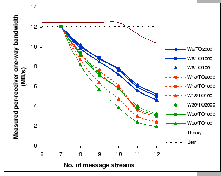
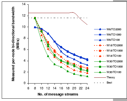
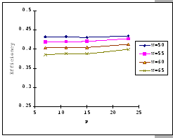
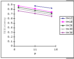
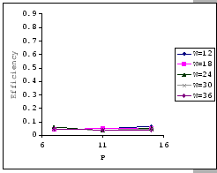
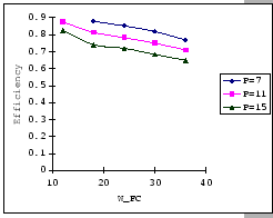
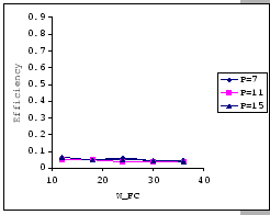
Figures 4.16 and 4.17 show the per-receiver bandwidths measured on the one-way and bi-directional tests with different window flow control and timeout settings. In general, the performance behaviors under such data flows agree with our conclusion made on the studies of the many-to-one congestion loss problem. Particularly, the test results match with our analyses that the flow control window size has the heaviest weight on the final performance, and the timeout setting comes next, while the number of attributed sources has the least weight. Furthermore, Figure 4.16 uncovers the intrinsic limitation of the uplink port, as the measurements show that it can only sustain at most 7 full FE message streams regardless of the window size setting. Once we move beyond its throughput limitation, the flow control setting becomes significant, and this indicates that the uplink port is now working under overload condition. Of the worst, Figure 4.17 further demonstrates that under heavy loading with bi-directional data flows, the circuitry of the uplink port cannot support more than 8 streams, i.e. only supports up to 4 concurrent duplex streams. Under such condition, both the data and control packets are subjected to lose as traffics on both directions are heavily congested, however, we still observe a similar congestion dynamic as identified in previous experiments. This fortifies our belief that the studies on the many-to-one congestion loss problem do capture those salient features of our GBN reliable transmission protocol.
![$\displaystyle T_{Eff}=\frac{E[y]*E[x]*g_{r}}{E[y]*E[S]+E[m]*TO}$](img202.png)
![$\displaystyle E[x]=\sum ^{\infty }_{n=1}(1-c)^{n-1}cn=\frac{1}{c}$](img221.png)
![$\displaystyle E[y]=\sum ^{\infty }_{h=1}a^{h-1}(1-a)h=\frac{1}{1-a}$](img224.png)
![$\displaystyle E[m]=\sum ^{\infty }_{q=1}(1-f)^{q-1}fq=\frac{1}{f}$](img226.png)