The ![]() parameter of our model provides two information related to the buffering
system: (1) it displays the maximum number of buffer units associated
to a switch's port, and (2) the associated buffering architecture
adopted by this switching unit. As the primary usage of providing
buffer storage is to handle temporary congestion, the natural starting
point of our investigation is to create artificial congestion problem.
For this communication microbenchmark, we carry out a set of tests
that systematically generate traffics from multiple input ports (S)
to a prefixed set of output ports (R). On each test, we start
with a short burst of packets (of predefined volume and packet size),
generated simultaneously from all the source nodes, and are flooded
to the target destination nodes (ports). After injecting the burst
into the network, all source nodes will stall for a specific duration,
which is long enough for the switch's buffers to clear off their loading
and for the receivers to count how many packets have they got. Then
the program increases the burst volume, and continues the same process
until the target burst volume is reached. By using different number
of source nodes (S) and sink nodes (R) on each test,
we collect a set of loss patterns which becomes the buffering signature
of the switching unit in question.
parameter of our model provides two information related to the buffering
system: (1) it displays the maximum number of buffer units associated
to a switch's port, and (2) the associated buffering architecture
adopted by this switching unit. As the primary usage of providing
buffer storage is to handle temporary congestion, the natural starting
point of our investigation is to create artificial congestion problem.
For this communication microbenchmark, we carry out a set of tests
that systematically generate traffics from multiple input ports (S)
to a prefixed set of output ports (R). On each test, we start
with a short burst of packets (of predefined volume and packet size),
generated simultaneously from all the source nodes, and are flooded
to the target destination nodes (ports). After injecting the burst
into the network, all source nodes will stall for a specific duration,
which is long enough for the switch's buffers to clear off their loading
and for the receivers to count how many packets have they got. Then
the program increases the burst volume, and continues the same process
until the target burst volume is reached. By using different number
of source nodes (S) and sink nodes (R) on each test,
we collect a set of loss patterns which becomes the buffering signature
of the switching unit in question.
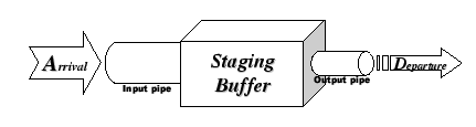
Before discussing on how to draw the conclusion from the buffering signature, we first illustrate the theory behind our microbenchmark. Assuming that the network is error-free, all packet losses are caused by buffer overflow, either in the switch port or at the receiver node. The prerequisite of having buffer overflow is the unbalance of flow across the buffer region, so we simplify the bottleneck region as a staging buffer between input and output pipes, as shown in Figure A.1.
Intuitively, the staging buffer starts queuing up data items when the departure rate is slower than the arrival rate. Thus, the ratio between the departure rate and arrival rate becomes a measure of congestion. Due to the limited size, this staging buffer cannot sustain long-term congestion, and eventually starts dropping all newly arrived packets when it is full.
Here we derive a deterministic model to delineate this overflow problem.
Let the staging buffer be of size ![]() units, and
the arrival and departure rates over this bottleneck stage be A
and D units per second respectively. Assume that at
units, and
the arrival and departure rates over this bottleneck stage be A
and D units per second respectively. Assume that at ![]() ,
the staging buffer is empty, and with an unbalance flow (
,
the staging buffer is empty, and with an unbalance flow (![]() ),
packets start to cumulate over the staging buffer. Now at
),
packets start to cumulate over the staging buffer. Now at ![]() ,
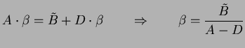
the buffer becomes full, then we have
,
the buffer becomes full, then we have
Therefore, when
![]() , the system can accommodate all
arrivals and the success probability is equal to one. However, after
buffer saturation, at
, the system can accommodate all
arrivals and the success probability is equal to one. However, after
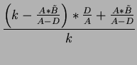
buffer saturation, at ![]() , newly arrived packets can only
be accepted and forwarded with a probability of
, newly arrived packets can only
be accepted and forwarded with a probability of
![]() .
Hence, we expect that the probability of success (
.
Hence, we expect that the probability of success (![]() ) on
moving k packets (where
) on
moving k packets (where
![]() ) across this bottleneck
stage when
) across this bottleneck
stage when ![]() is:
is:
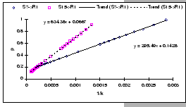
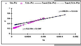
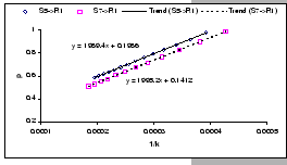
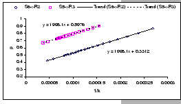
We see from equation (A.2) that by varying these parameters, we are expecting to get different packet loss ratio:
|
|
[IBM 8275-326 (Input-buffered)]
 [IBM 8275-326 (Input-buffered)] [IBM 8275-326 (Input-buffered)]
[Cisco 2980G (Output-buffered)]
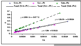 [Cisco 2980G (Output-buffered)] [Cisco 2980G (Output-buffered)]
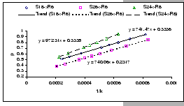
[Intel 510T (Shared-buffered)]
 [Intel 510T (Shared-buffered)] [Intel 510T (Shared-buffered)]
|