In Chapter 5, we have presented the Synchronous Shuffle complete
exchange algorithm, which is a bandwidth-optimal algorithm on any
non-blocking network. The spirit of this algorithm is the node contention-free
schedule operated at the packet level without explicit synchronization
operation. By effectively utilizing the send and receive channels,
this scheme multiplexes all the messages seamlessly to a single pipeline
flow by scheduling consecutive packets to different destination nodes
according to a node contention-free permutation (![]() ).
).
If every operation is executed on schedule, the permutation scheme of the synchronous shuffle exchange can be finished in minimal time. However in reality, as this schedule induces intensive communications and demands on logical synchrony, any non-deterministic delays between events could break the synchronism and result in congestion developed in the switch. For example, non-coordinated process scheduling would introduce randomness. We have shown in previous chapter that not all switches can withstand such an intensive communication pattern for an extended period.
Generally, having logical synchrony on all cluster nodes is an idealistic assumption for the case of commodity clusters, which have no hardware synchronization support. To impose this synchrony, explicit synchronization operations can be used. However, this brings on extra synchronization overhead to the total communication time, and also stalls the communication pipelines as no data communications are taking place during synchronization. Since performance loss is caused by oversubscription to the network, which induces packet loss at the bottleneck region, the best solution to avoid congestion loss is to prevent oversubscription to the network. That can be done by applying some form of traffic control on each node to minimize the contention problem.
The conjecture behind the contention problem induced by the synchronous shuffle exchange algorithm is the non-deterministic delays on communication events. With the hierarchical network, two more sources of delay could contribute to this non-determinism.
In this study, we adopt a proactive approach in the congestion control. This congestion control scheme is different from traditional approaches. Conventional mechanisms for controlling congestion are based on end-to-end windowing schemes [89], however, they are not suitable for collective operations in high-speed networks. This is because they are usually reactive schemes. They probe for congestion signals, such as packet loss and timeout signals, and respond by recovering the loss and regulating the traffic load to avoid further loss. However, we have already lost some packets, and this has affected the performance. Our GBN reliable protocol described in Chapter 4 is an example of a reactive scheme. Besides, the feedback information from the network is usually outdated due to the propagation and transmission delays. Hence, any reactive action taken may be too late to avoid further loss. Furthermore, end-to-end windowing only provides traffic information on individual connection. It lacks in a global picture of the network, such as the number of traffic sources and the communication pattern in used.
However, in cluster computing, the traffic pattern is predictable
in the case of collective operations on an enclosed network. Therefore,
we can utilize those available information, such as the network buffer
capacities (![]() ) of the switched network, the communication
pattern and communication volume, to derive some resource-aware congestion
control scheme. With our global congestion control scheme, each source
is assigned with a predefined resource limit, and our scheme forces
them to regulate their traffic loads below this limit. By having a
fair share of resources, this ensures that no source will exceed its
allowed traffic capacity and avoids congestion loss.
) of the switched network, the communication
pattern and communication volume, to derive some resource-aware congestion
control scheme. With our global congestion control scheme, each source
is assigned with a predefined resource limit, and our scheme forces
them to regulate their traffic loads below this limit. By having a
fair share of resources, this ensures that no source will exceed its
allowed traffic capacity and avoids congestion loss.
We have observed that during the execution flow, at ![]() communication step, a process is sending a data packet to another
process according to the node contention-free permutation scheme
communication step, a process is sending a data packet to another
process according to the node contention-free permutation scheme ![]() .
If every operation is on schedule, the number of outstanding data
packets (
.
If every operation is on schedule, the number of outstanding data
packets (![]() ) in transit from a process to other process
is bounded by
) in transit from a process to other process
is bounded by
![]() . Under
mild congestion, the process experiences slight increase of
. Under
mild congestion, the process experiences slight increase of ![]() .
If congestion persists, this eventually induces packet loss, and
.
If congestion persists, this eventually induces packet loss, and ![]() will increase considerably. The above observation implies that to
avoid overflowing the network buffers, we need to regulate the number
of outstanding packets (
will increase considerably. The above observation implies that to
avoid overflowing the network buffers, we need to regulate the number
of outstanding packets (![]() ).
).
The principle behind our congestion control scheme is quite simple.
When applying this scheme on our complete exchange algorithm, all
senders are assigned with a global window (![]() ) at the beginning
of the communication event. This
) at the beginning
of the communication event. This ![]() factor acts as a controller
to limit the amount of traffic that a particular sender can inject
into the network. If a sender finds that sending out a data packet
may overload the network, when
factor acts as a controller
to limit the amount of traffic that a particular sender can inject
into the network. If a sender finds that sending out a data packet
may overload the network, when
![]() , it just halts current
transmission and waits until it is safe to transmit, i.e.
, it just halts current
transmission and waits until it is safe to transmit, i.e.
![]() .
By picking the correct value for
.
By picking the correct value for ![]() , this scheme guarantees
that during any interval, the total number of packets entering the
network does not exceed the sum of a pre-specified limit, which is
the network buffer capacity at the bottleneck region. To compute
, this scheme guarantees
that during any interval, the total number of packets entering the
network does not exceed the sum of a pre-specified limit, which is
the network buffer capacity at the bottleneck region. To compute ![]() ,
we need to identify the bottleneck region and measure the buffer capacity
(
,
we need to identify the bottleneck region and measure the buffer capacity
(![]() ) associated to the bottleneck, then we derive
) associated to the bottleneck, then we derive ![]() from
from ![]() on the principle of fair sharing.
on the principle of fair sharing.
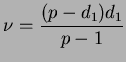
Based on the communication pattern and schedule, we estimate the average
number of packets (![]() ) generates at each communication step
which are forwarded to the bottleneck region. Without lost of generality,
let's take the FE/GE hierarchical network as an example. Assume that
the uplink ports are the critical bottlenecks and they are of input-buffered
architecture. Under the synchronous shuffle schedule, in p-1
communication steps, a process generates p-1 data packets which
are destined to p-1 distinct nodes. However, only
) generates at each communication step
which are forwarded to the bottleneck region. Without lost of generality,
let's take the FE/GE hierarchical network as an example. Assume that
the uplink ports are the critical bottlenecks and they are of input-buffered
architecture. Under the synchronous shuffle schedule, in p-1
communication steps, a process generates p-1 data packets which
are destined to p-1 distinct nodes. However, only ![]() packets are switched locally, and the rest,
packets are switched locally, and the rest, ![]() packets,
are forwarded by the Fast Ethernet switch to its uplink port. Therefore,
there are
packets,
are forwarded by the Fast Ethernet switch to its uplink port. Therefore,
there are
![]() packets being forwarded upstream by
each FE switch in p-1 communication steps. Based on the node
contention-free permutation, the same amount of data packets are switched
from the Gigabit backbone back to each FE switch. Thus, the average
number of data packets directed to each uplink port per communication
step is
packets being forwarded upstream by
each FE switch in p-1 communication steps. Based on the node
contention-free permutation, the same amount of data packets are switched
from the Gigabit backbone back to each FE switch. Thus, the average
number of data packets directed to each uplink port per communication
step is
 |
(6.1) |
From this, we derive the value of ![]() , which is
, which is
 |
(6.2) |
However, knowing the value of ![]() is a necessary but not
sufficient condition to avoid congestion loss. This is because
is a necessary but not
sufficient condition to avoid congestion loss. This is because ![]() is derived from taking the average traffic load, and unlike traditional
end-to-end scheme, global windowing needs to monitor and regulate
all traffic flows of a process, not just one connection. If the traffic
distribution is not uniformly spread across the network, the global
windowing scheme could not fulfill its function correctly. This is
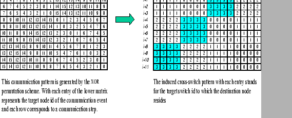
being shown in Figure 6.3. In this example, we assume that
the bottleneck region of the 4X4 two-level hierarchical network
is at the uplink ports with
is derived from taking the average traffic load, and unlike traditional
end-to-end scheme, global windowing needs to monitor and regulate
all traffic flows of a process, not just one connection. If the traffic
distribution is not uniformly spread across the network, the global
windowing scheme could not fulfill its function correctly. This is
being shown in Figure 6.3. In this example, we assume that
the bottleneck region of the 4X4 two-level hierarchical network
is at the uplink ports with ![]() . However, under the XOR
permutation scheme, we could experience the contention loss problem
even though global windowing is adopted.
. However, under the XOR
permutation scheme, we could experience the contention loss problem
even though global windowing is adopted.
In this example, the size of ![]() is
is
![]() .
Assume that at communication step i, four packets originate
from switch 2 and head for switch 3 are blocked by some cause, e.g.
HOL, so as those packets that follow in step i+1, i+2,
and i+3 from the same switch. However, no process is aware
of the congestion problem unless their global windows become saturated.
This may only be happened until step i+8 when processes in
switch 3 detect the congestion problem. By that time, processes in
switch 1 have already sent out all their packets to processes in switch
3, which further increases the queue length at switch 3. Moreover,
processes in switch 0 are not aware of the problem. This is because
global windowing collects traffic information on the base of past
events, but none of these past events could indicate the congestion
problem in switch 3. As a result, processes in switch 0 continue to
send all their packets to processes in switch 3, which finally overflow
the buffer.
.
Assume that at communication step i, four packets originate
from switch 2 and head for switch 3 are blocked by some cause, e.g.
HOL, so as those packets that follow in step i+1, i+2,
and i+3 from the same switch. However, no process is aware
of the congestion problem unless their global windows become saturated.
This may only be happened until step i+8 when processes in
switch 3 detect the congestion problem. By that time, processes in
switch 1 have already sent out all their packets to processes in switch
3, which further increases the queue length at switch 3. Moreover,
processes in switch 0 are not aware of the problem. This is because
global windowing collects traffic information on the base of past
events, but none of these past events could indicate the congestion
problem in switch 3. As a result, processes in switch 0 continue to
send all their packets to processes in switch 3, which finally overflow
the buffer.
An obvious reason for this failure is that the feedback information on traffic condition is not regularly gathered from all part of the network. Thus, information on part of the network is outdated. Although the overflow situation could be detected and resolved by both global windowing and individual end-to-end flow control scheme, performance has been suffered as packets are lost inevitably. If we can arrange all communication events in a way that each process is communicating with different processes reside in a node linked to different switches at each communication step. Then, the traffic loads would become more evenly distributed as well as having more regular information feedback between different processes in different part of the network.
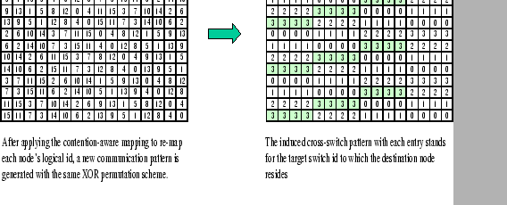
An approach in generating this kind of dispersive pattern is by adopting
a contention-aware permutation, which includes knowledge on the network
constraints to generate the communication schedule. Observed that
the original permutation is obtained by some simple functions (![]() )
which operate on inputs such as current communication step and node
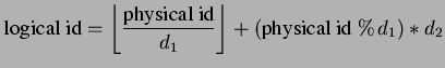
id. A simple method to incorporate the network structure into the
original permutation is by redefining a mapping between the logical
node id to its physical id. One example of such permutation scheme
(
)
which operate on inputs such as current communication step and node
id. A simple method to incorporate the network structure into the
original permutation is by redefining a mapping between the logical
node id to its physical id. One example of such permutation scheme
(![]() ) can be as follows:
) can be as follows:
|
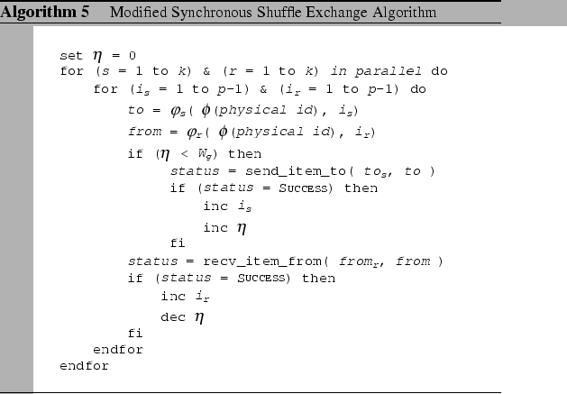
Based on the global windowing and the contention-aware permutation
scheme, we have modified the synchronous shuffle exchange algorithm
to work efficiently on the two-level hierarchical network, and the
modified algorithm is given in Algorithm 5.