6.3 Experimental Analyses

Our experimental platform is a cluster consists of 32 standard PCs running Linux 2.2.14. Each cluster node equips with a 733MHz Pentium III processor with 256KB L2 cache, 128MB of main memory, an integrated 3Com 905C FE controller and is connected to the Ethernet-based switched network. Once again, we use the Directed Point communication system to drive the network and conduct all our experiments. In this study, we use four Fast Ethernet switches and one Gigabit Ethernet switch to set up various configurations to evaluate our algorithm.

The GE backbone switch is a chassis switch from Alcatel. It is the model PowerRail 2200 (PR2200) with backplane capacity reaches 22 Gigabit per second (Gbps). This switch is equipped with 8 GE ports on 2 modules, but we only use at most 4 ports in our experiments. Four FE switches are from IBM, which are of the model 8275-326. It is a 24-port input-buffered switch with backplane capacity reaches 5 Gbps. A one-port GE uplink module is installed on each FE switch for connecting to the Gigabit backbone switch. Table 6.1 summaries all the buffer parameters of the above switches, which are used in our algorithm to compute the global windows ($W_{g}$) on different network configurations.

Table 6.1: The $B_{L}$ parameter of different switches in our experimental setup

Switch/uplink	Architecture	$B_{L}$
Alcatel PR2200	Shared-buffered	820
IBM 8275-326	Input-buffered	43
IBM GE uplink	Input-buffered	45

To analyze and evaluate the performance of our congestion control mechanism, we have set up five different configurations on this cluster - 16X1, 8X2, 8X3, 6X4 and 8X4, with each configuration corresponds to a different degree of contention on the uplink ports (except configuration 16X1). The configuration AXB corresponds to connect A cluster nodes to each FE switch, and there are total B FE switches interconnected by the GE switch. This makes up a cluster size of $A*B$ nodes.

6.3.1 16-Node Single Switch - 16X1

The synchronous shuffle exchange is designed to work efficiently on any non-blocking network. However, in previous chapter, we have shown that there is internal constraint on an input-buffered switch, which limits the problem size scalability of our synchronous shuffle exchange algorithm. Although group shuffle exchange is devised to alleviate the problem, it only works sub-optimally from the analytical point of view. In this chapter, we have devised a new congestion control scheme to make synchronous shuffle exchange works efficiently on the hierarchical network. We consider that the same congestion control scheme can be applied to the single-router network to offset the limitation imposed by the HOL blocking.

Figure 6.5: Performance of modified synchronous shuffle exchange on a single input-buffered switch. (Legends: sync - synchronous shuffle; pair - pairwise; GW - global windowing)

[Measured execution time]

[Achieved bandwidth]

Figure 6.5 presents the measured results of four complete exchange implementations on a 16-node cluster interconnected by a single input-buffered switch (IBM 8275-326). They are the synchronous shuffle with global windowing (sync+GW), the pairwise exchange (pair), the original MPICH implementation (MPICH) and the pairwise exchange MPI implementation (pair-MPI). The experiment is conducted with each node sending a long message to every node in the cluster, which ranges from 1 KB to 1200 KB of data to each node. Both the measured performance and the per-node achieved bandwidth of each implementation are shown in the graphs.

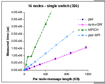
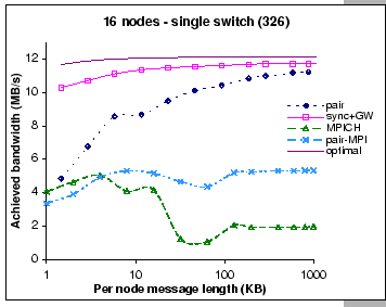
We have shown in Figure 5.6 (Section 5.4) that the performance of the original synchronous shuffle algorithm degrades significantly after k>512, which corresponds to a message length of 746 KB per node. By supplementing the synchronous shuffle algorithm with the global windowing scheme, we show that it continues to operate efficiently as the problem size scales. When compared to the optimal performance (Eq. 5.3), the modified synchronous shuffle exchange algorithm has its efficiency ranged from 87% to 97% of the theoretical bandwidth. When compared with the pairwise exchange, the results show that the modified synchronous shuffle algorithm can effectively mask away synchronization overhead and achieves better performance. This shows that the add-on congestion control scheme does not affect the efficiency of our synchronous shuffle exchange algorithm. Indeed, it effectively guards against the congestion loss.

Not to mention on the poor performance of both MPI implementations, even though we are now using a faster processor and pumping the network with more data, their performances are restrained by the high protocol overheads. Although the pairwise MPI implementation generally performs better than the original MPICH implementation, we observe that the original MPICH implementation is slightly better on small message exchanges. This reflects that the use of non-blocking send and receive operations could hide away part of the synchronization overhead when exchanging small size messages and the induced contention problem is minimal, e.g. the use of eager protocol in the MPICH. However, when exchanging long messages, it would be better to have a well-coordinated schedule.

6.3.2 16-Node Hierarchical Configuration - 8X2

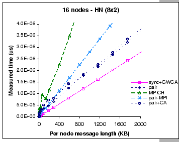
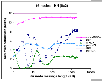
In this subsection, we start our experiments on the hierarchical network by first using a 16-node configuration. We are using two Fast Ethernet switches with eight nodes connect to each switch, and they are interconnected via the Gigabit Ethernet switch. With this setup, the theoretical bisection bandwidth [46] is 1 Gb/s, which should be sufficient for the current cluster configuration.

6.3.2.0.1 Baseline Studies

Figure 6.6: The achieved performance of the 10X2 hierarchical network under multiple bidirectional message exchanges. (Legends: cross-switch - measured aggregated bandwidth over the hierarchical network; local - measured aggregated bandwidth on the single switch)

Our experiment results in Section 4.3.4 have shown that the uplink circuitry of the IBM 8275-326 switch is not as good as it claims. In order to reason on the measured performance, such that we can make the correct judgment on the performance of our implementations, we have performed some baseline measurements to determine the best achievable throughput across these GE uplinks. Instead of using the 8X2 configuration, we have the 10X2 configuration and measure the achieved aggregated bandwidth across the hierarchical network by having multiple concurrent bi-directional data exchanges. Figure 6.6 shows the results of this baseline study. The peak aggregated bandwidth achieved on this setting is 103 MB/s with 12 concurrent bi-directional flows across the uplink ports. Beyond that, the communication performance starts to deteriorate gradually. With the same software and hardware settings, but replacing the hierarchical network with a single IBM 8275-326 switch, we can achieve a linearly scaled aggregated bandwidth, which is labeled as ``local'' in the graph. This demonstrates that the limitation is on the uplink circuitry, not on other components. With this baseline measurement, we have a solid foundation to justify on the expected communication efficiency across the problematic uplink ports, such that we have

$$\textrm{Best cross switch data exchange time}=\frac{\textrm{Total cross switch volume}}{103\: MB/s}$$ (6.4)

Take an example with the 8X2 configuration, the total cross-switch volume on the k-item complete exchange is $2k*\textrm{MTU}*(16-d_{1})*d_{1}$ bytes. Thus, the best timing in delivering this volume of data across the uplink connection is $\frac{128*k*\textrm{MTU}}{103}$seconds. Assumed that an efficient communication schedule should be able to arrange all local and cross-switch communications be happened concurrently. Therefore, the execution time of the k-item complete exchange should be bounded by the best cross-switch data exchange time. Then, the best achieved per-node bandwidth for this k-item complete exchange operation is $\frac{k*\textrm{MTU}*15}{\frac{128*k*\textrm{MTU}}{103}}=12.07\textrm{ MB}/s$.

$\qquad$

Figure 6.7: The performance of modified synchronous shuffle exchange on the 8X2 configuration - 8 nodes connect to each FE switch, which is connected to the PR2200. (Legends: GWCA- global windowing plus contention-aware permutation scheme; CA-contention-aware permutation scheme only)

[Measured execution time]

[Achieved bandwidth]

After understanding about the performance limitation of the network, we carry on with our analysis. With the 8X2 configuration, the theoretical computed value of $W_{g}$ is 10; however, when considered together with implementation issue, such as the existence of control packets with reliable support, the calculated value of $W_{g}$ is $\left\lfloor 45\div \frac{(16-8)*8*2}{15}\right\rfloor =5$. We have measured the performance of the modified synchronous shuffle algorithm with this global windowing setting, and the results are presented in Figure 6.7. Similarly, we are comparing different implementations of the complete exchange operation on this configuration. Five sets of measurements are shown in the graphs. They are the synchronous shuffle with global windowing and contention-aware permutation (sync+GW+CA), pairwise exchange (pair), pairwise exchange with contention-aware permutation (pair+CA), the original MPICH implementation and the pairwise exchange MPI implementation (pair-MPI). The results show that synchronous shuffle exchange with global windowing and contention-aware permutation performs the best amongst all tested implementations in this configuration. When compared to the expected best achievement, the modified synchronous shuffle shows its effectiveness in utilizing the network pipelines as well as avoiding the congestion loss, since it reaches 93% of the best achieved performance.

However, we find that the performance of the DP pairwise exchange implementation has degraded considerably under this hierarchical configuration when compared to its performance on the single-switch case (Figure 6.5b). Initially, the performance of the DP pairwise implementation (labeled as ``pair'') increases with the increase in message length until the maximum capacity of the uplink ports has reached. After that, the performance is affected by the congestion loss problem. However, our GBN reliable protocol could only recover from the loss with long message exchanges. This is being shown as the slow increased in the achieved bandwidth after experiencing the congestion loss problem. To investigate on whether the contention-aware permutation scheme would also benefit the pairwise exchange algorithm, we have applied the same contention-aware permutation on the DP pairwise implementation. The measured results (labeled as ``pair+CA'') show that this augmentation exhibits a similar behavior as compared to the pure pairwise exchange. However, the congestion loss problem appears earlier than we have expected, and the overall performance is slightly worse than the pure pairwise exchange implementation.

On the other hand, it is interested to see that the performances of the two MPI implementations do not have significant performance changes on this hierarchical configuration. We find that they both have slight improvements on exchanging long message, but the original MPICH implementation has lost its performance on exchanging small messages. This could be the result of contention over the uplinks as the MPICH implementation does not carefully schedule those communication events. This indicates that under this hierarchical configuration, it demands for a better communication scheme to coordinate the communication events, since the performance is limited by the aggregated bandwidth.

6.3.3 24-Node Hierarchical Configurations - 8X3 and 6X4

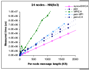
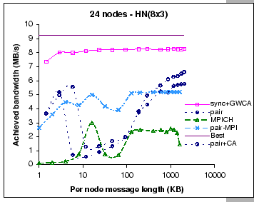
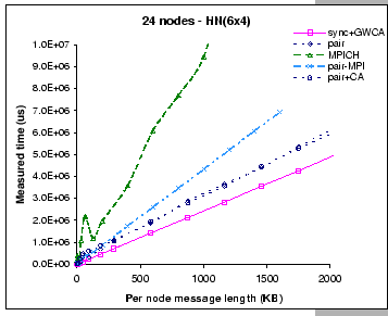
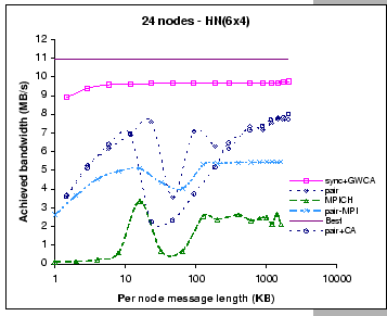
To construct a 24-node cluster with our hardware resources, we can arrange the hierarchical network in two different configurations:

1. 8X3 - By connecting three Fast Ethernet switches to the Gigabit Ethernet switch, and each FE switch has eight cluster nodes connected to it, we get a 24-node cluster. With this configuration, the computed value of $W_{g}$ is 4 and the experimental results are shown in Figure 6.8.

   Figure 6.8: Performance of different complete exchange implementations on the 8X3 hierarchical configuration

   [Measured execution time]

   [Achieved bandwidth]

2. 6X4 - All four FE switches are connected to the GE switch with six cluster nodes attached to each FE switch, we have the second 24 nodes configuration. With this configuration, the computed value of $W_{g}$ is 5 and the experimental results are shown in Figure 6.9.

   Figure 6.9: Performance of different complete exchange implementations on the 6X4 hierarchical configuration

   [Measured execution time]

   [Achieved bandwidth]

We have performed the same set of tests on these two configurations as compared to the 8X2 setup. When comparing their expected best achievements on these two configurations, which are of 9.25 MB/s on the 8X3 configuration and of 10.96 MB/s on the 6X4 configuration, we see that the 6X4 configuration has a better throughput performance. This is reasonable since we only attach 6 nodes to each FE switch on the 6X4 setup. Again, we see that the modified synchronous shuffle performs the best on both setups; however, it only reaches 89% and 88% of the expected best achievements on the 8X3 and 6X4 configurations respectively. A possible explanation on the performance degradation is due to the use of small global window settings, which may reduce the pipelining efficiency. However, increase the global window size would increase the congestion loss probability, this could create an adverse effect on the overall performance.

As for the two MPI implementations, their measured performance look similar to the performance observed in the 8X2 configuration. Such that the achieved bandwidth of the pairwise MPI implementation is peaked at 5.4 MB/s and 5.2 MB/s on 6x4 and 8x3 respectively, as compared to 5.5 MB/s on the 8X2 setup. Similarly, the achieved bandwidth of the MPICH implementation is peaked at 2.7 MB/s and 2.6 MB/s on 6X4 and 8X3 respectively, while it achieves 2.7 MB/s on the 8X2 setup. Besides, we observe that as the cluster size has increased from 16 nodes to 24 nodes, the observed contention problem of the original MPICH implementation on small message exchanges is getting worse than the 8X2 configuration. Nevertheless, all these findings support our belief that conventional communication libraries are restrained by the high software overheads.

As for the DP pairwise implementations, their measured results exhibit different performance behaviors on these two configurations. On a configuration that supports less aggregated bandwidth (8X3), we find that we have experienced severe performance loss starting at small size message exchanges. But, with a less restrictive configuration (6X4), the losses start to appear only on medium size message exchanges. After that, the performance slowly increases when exchanging longer messages. On the other hand, we find that the add-on contention-aware scheme (pair+CA) performs better on the 8X3 configuration when compared to the pure pairwise implementation. A possible explanation to this observation is that the contention-aware scheme is more effective when operates on a more stringent configuration.

6.3.4 32-Node Hierarchical Configuration - 8X4

Figure 6.10: Performance of different complete exchange implementations on the 8X4 hierarchical configuration

[Measured execution time]

[Achieved bandwidth]

With this configuration, we interconnect four FE switches to the GE switch, and each FE switch is attached with 8 cluster nodes. Carry on with the same set of experiments with the global windowing parameter ($W_{g}$) set to 3, the measured results are shown in Figure 6.10. Same as other experiments, the modified synchronous shuffle algorithm shows its clear advantage over other implementations when running on this hierarchical configuration. In particular, it achieved per-node bandwidth peaks at 7.67 MB/s, which is around 92% of the expected best achievement (8.32 MB/s) on this configuration.

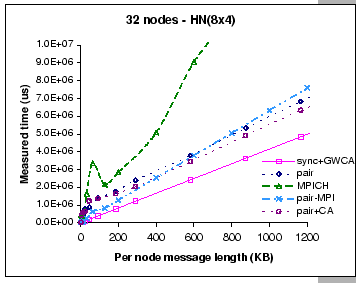
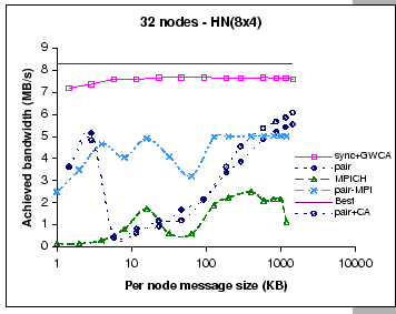
As for the two MPI implementations, their performances closely match with other configurations, which are peaked at 2.5 MB/s on the per-node bandwidth for the MPICH implementation and 5.03 MB/s on the pairwise MPI implementation. However, the performance of our DP pairwise exchange implementation suffers considerably when exchanging small to medium size messages, as the results show that the pairwise MPI implementation outperforms the DP pairwise implementations on this message range. This indicates that our GBN reliable protocol is not working as effectively as the TCP protocol except with large message exchanges. Once again, we observe that the add-on contention-aware permutation on the pairwise implementation has slight performance improvement on the current configuration. When compared this finding with the results on other configurations, we believe that the contention-aware scheme works better on a more stringent configuration. This observation shows that contention-aware permutation alleviates the congestion build-up at the uplink ports; however, it still has to work together with the global windowing scheme in order to avoid congestion loss.